
Diagnostic Test Accuracy Meta-Analysis
Diagnostic-Test-Accuracy.Rmdmars_dta() jointly pools sensitivity and specificity for
a single index test. Supply one row per independent study with the four
counts from its 2-by-2 table against a reference standard. This example
uses fictional studies.
library(mars)

studies <- data.frame(
  study = sprintf("s%02d", 1:16),
  TP = c(44, 50, 56, 59, 64, 68, 69, 71, 52, 58, 61, 65, 70, 74, 75, 77),
  TN = c(52, 42, 62, 74, 53, 65, 59, 72, 52, 76, 59, 47, 69, 80, 65, 62),
  setting = rep(c("clinic", "community"), 8)
)
studies$FN <- 80L - studies$TP
studies$FP <- 90L - studies$TN
head(studies)
## study TP TN setting FN FP
## 1 s01 44 52 clinic 36 38
## 2 s02 50 42 community 30 48
## 3 s03 56 62 clinic 24 28
## 4 s04 59 74 community 21 16
## 5 s05 64 53 clinic 16 37
## 6 s06 68 65 community 12 25Fit a bivariate model
## Bivariate diagnostic accuracy meta-analysis (gaussian REML)
## 16 studies, 0 corrected strata, 0 omitted studies
##
## Pooled accuracy (95% confidence intervals)
##  profile    endpoint  estimate     lower     upper
##        1 sensitivity 0.8072093 0.7416975 0.8592585
##        1 specificity 0.6948209 0.6309423 0.7519891
##
## Between-study covariance on the logit scale
##             sensitivity specificity
## sensitivity   0.4920799   0.2071295
## specificity   0.2071295   0.2839586
## Between-study correlation: 0.5541108
The default Gaussian REML model fits a mean logit for each endpoint. The reported operating point transforms those two fitted means back to probabilities. Its confidence intervals describe uncertainty about the operating point. Use prediction intervals to include the estimated between-study heterogeneity and describe the underlying sensitivity and specificity of a new study.
predict(fit, interval = "prediction")## profile endpoint logit estimate lower upper
## 1 1 sensitivity 1.4319776 0.8072093 0.5015747 0.9457131
## 2 1 specificity 0.8227554 0.6948209 0.4353030 0.8705418fit$tau is the estimated between-study covariance of the
two logits. The unstructured default estimates both endpoint variances
and their covariance. structure = "DIAG1" estimates both
variances and sets the covariance to zero. fit$fit contains
the underlying multivariate mars object.
plot(fit)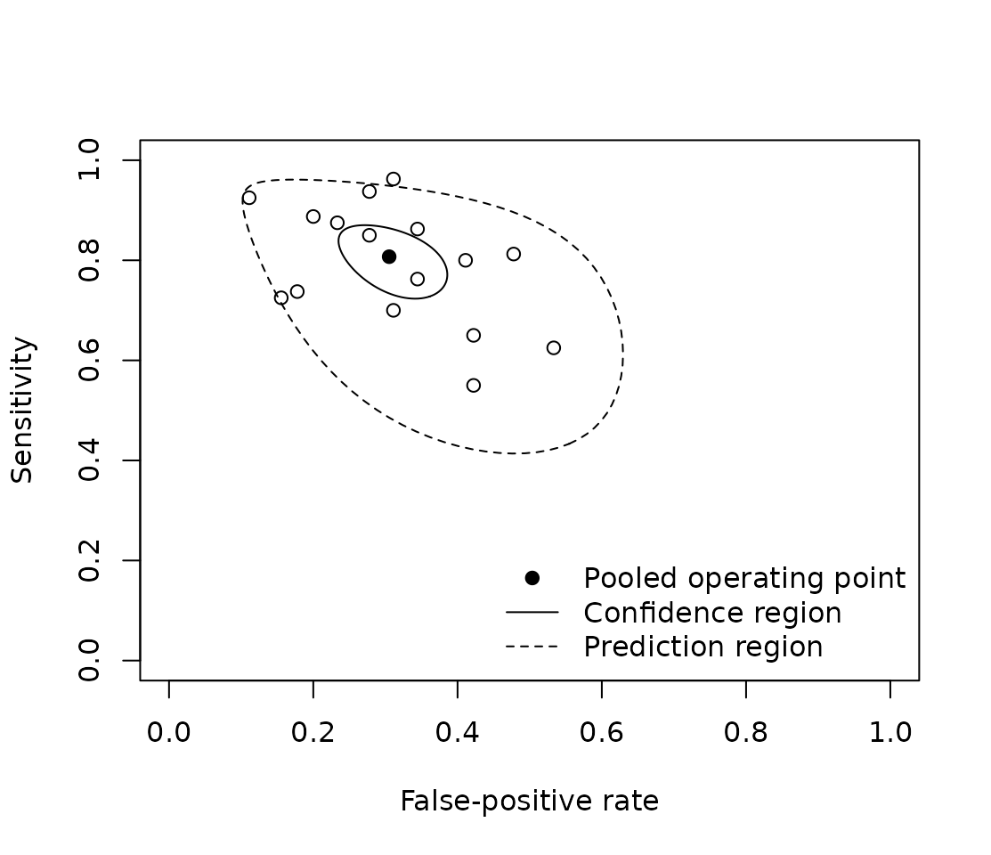
The plot shows each study’s raw sensitivity and false-positive rate (1 − specificity). The two regions use the joint logit-scale covariance and are back-transformed to ROC axes. The prediction region treats the estimated heterogeneity covariance as fixed.
Examine a study-level moderator
Use a one-sided formula. Each endpoint gets its own coefficient for each moderator, so the change in sensitivity can differ from the change in specificity. Supply moderator values to obtain fitted operating points.
by_setting <- mars_dta(studies, studyID = "study", moderators = ~ setting)
profiles <- data.frame(setting = c("clinic", "community"))
predict(by_setting, newdata = profiles)
## profile endpoint logit estimate lower upper
## 1 1 sensitivity 1.2852721 0.7833459 0.6784133 0.8610519
## 2 1 specificity 0.6489676 0.6567778 0.5624867 0.7401358
## 3 2 sensitivity 1.5905626 0.8306952 0.7389743 0.8947759
## 4 2 specificity 1.0039488 0.7318343 0.6449932 0.8038913The profile column indexes the rows of
newdata. For a ROC plot of a moderated fit, supply a single
profile.
Inspect sampling variances and zero-cell corrections
Sensitivity is calculated from TP and FN, and specificity from TN and FP. The logit of each proportion is the log ratio of its two cells. Its approximate sampling variance is the sum of the reciprocals of those cells. Because the two proportions are estimated in disjoint strata, conditional on the stratum totals, their within-study sampling covariance is zero. The fitted between-study covariance describes how the two true logits vary together across studies.
By default, if a stratum contains a zero, 0.5 is added to both cells in that stratum for the logit and variance calculations. The raw counts are retained.
sparse <- studies
sparse[1, c("TP", "FN")] <- c(0L, 20L)
corrected <- mars_dta(sparse, studyID = "study")
subset(corrected$effects, study_id == "s01")
## study_id endpoint events failures total corrected yi vi
## 1 s01 sensitivity 0 20 20 TRUE -3.7135721 2.04878049
## 2 s01 specificity 52 38 90 FALSE 0.3136576 0.04554656A stratum with a zero total has no information about that endpoint
and is rejected. Missing counts or moderators raise an error by default.
Set missing = "omit" to omit whole incomplete studies and
inspect omitted_studies. Study identifiers must be present
and unique in either case.
Fit the binomial model with a zero cell
The Gaussian approximation can be sensitive to the correction when
counts are sparse. With family = "binomial", Mars fits the
original TP and TN counts conditional on their stratum totals. It
estimates the correlation between the two study-level random effects and
integrates them out using adaptive Gauss–Hermite quadrature. The
binomial model uses maximum likelihood.
binomial <- mars_dta(sparse, studyID = "study", family = "binomial")
subset(binomial$effects, study_id == "s01")
## study_id endpoint events failures total corrected
## 1 s01 sensitivity 0 20 20 FALSE
## 2 s01 specificity 52 38 90 FALSE
predict(binomial)## profile endpoint logit estimate lower upper
## 1 1 sensitivity 1.3640011 0.7964092 0.6849298 0.8756081
## 2 1 specificity 0.8358514 0.6975907 0.6348662 0.7537201Study s01 contributes 0 true positives out of
20 to the binomial likelihood. Its sensitivity row retains zero
events and reports corrected = FALSE. Both
reference-standard strata still need positive totals in every study. The
model also needs at least one success and one failure for each endpoint
across the included studies.
The quadrature argument controls the number of
integration nodes per dimension. You can increase it to check numerical
stability in a sparse or heterogeneous dataset. Both models require one
table per study. Paired tests and multiple thresholds reported within
the same study require information about their sampling dependence.
Draw a summary ROC curve
Both the Gaussian and binomial fits support a Rutter–Gatsonis summary ROC curve. It traces sensitivity over false-positive rates as the latent threshold varies at the profile’s mean accuracy. Each curve passes through the pooled operating point, and its slope on the logit scale is the ratio of the two between-study standard deviations.
plot(binomial, sroc = TRUE)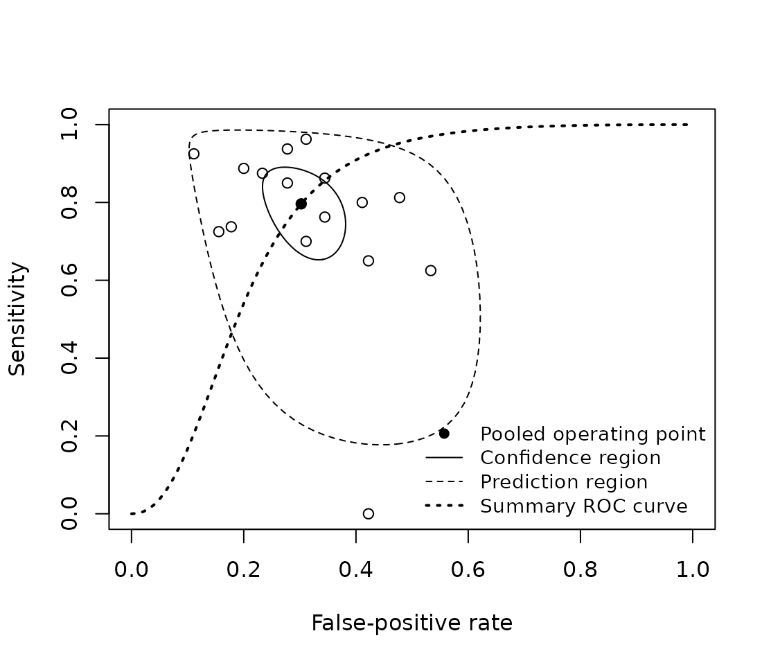
Use dta_sroc() to obtain coordinates on a custom grid.
Here the Gaussian and binomial fits both use the same studies with the
zero cell.
##   profile fpr sensitivity
## 1       1 0.2   0.6637980
## 2       1 0.3   0.8031559
## 3       1 0.4   0.8809184
dta_sroc(binomial, fpr = rates)## profile fpr sensitivity
## 1 1 0.2 0.5404343
## 2 1 0.3 0.7923267
## 3 1 0.4 0.9091882For a moderated fit, each row of newdata specifies one
curve. The moderators shift the pooled operating point while the
logit-scale slope is shared across profiles. Every moderator is held
fixed, including any measured threshold in the formula. To examine the
fitted association with a measured threshold, use predict()
to compare pooled operating points at different threshold values. To
overlay a curve on the ROC plot, choose one profile.
dta_sroc(by_setting, newdata = profiles, fpr = rates)## profile fpr sensitivity
## 1 1 0.2 0.5701717
## 2 1 0.3 0.7341058
## 3 1 0.4 0.8343010
## 4 2 0.2 0.7447101
## 5 2 0.3 0.8585864
## 6 2 0.4 0.9171671Interpret the curve over the range of false-positive rates supported by the studies. Rates outside that range are extrapolations.
Prepare effects for two paired tests
When the same participants take two tests, report the joint test
results separately for the diseased and non-diseased participants. In
the example below, pn = 10 in the diseased stratum means 10
participants were positive on test A and negative on test B.
paired <- data.frame(
  study_id = "s01",
  stratum = c("diseased", "non_diseased"),
  pp = c(30, 5), pn = c(10, 10), np = c(5, 15), nn = c(5, 70)
)

prepared <- dta_paired_effects(paired, tests = c("A", "B"))
prepared$effects[c("effect_id", "events", "total", "yi", "vi")]
## effect_id events total yi vi
## 1 A:sensitivity 40 50 1.3862944 0.12500000
## 2 A:specificity 85 100 1.7346011 0.07843137
## 3 B:sensitivity 35 50 0.8472979 0.09523810
## 4 B:specificity 80 100 1.3862944 0.06250000
round(prepared$sampling_covariance[["s01"]], 4)## A:sensitivity A:specificity B:sensitivity B:specificity
## A:sensitivity 0.1250 0.0000 0.0238 0.0000
## A:specificity 0.0000 0.0784 0.0000 0.0098
## B:sensitivity 0.0238 0.0000 0.0952 0.0000
## B:specificity 0.0000 0.0098 0.0000 0.0625The block contains one sampling covariance between the two logit sensitivities and another between the two logit specificities. Sensitivity and specificity use disjoint reference-standard strata, so the corresponding cross-stratum sampling covariances are zero. The helper prepares the effects and covariance as standalone outputs.
An empty joint cell is valid if each test still has both positive and
negative results in its stratum. If a marginal count is zero,
zero_cell = "add_half" adds 0.5 to all four joint cells in
the affected stratum. This gives both tests a common corrected joint
table for the logits and their covariance. The raw table and amount
added per cell are recorded in prepared$joint_counts.
Pool paired accuracy and compare the tests
mars_dta_paired() uses the same joint-count format to
fit a Gaussian multivariate model. Here are 24 fictional studies. The
probabilities used to generate the joint counts vary across studies, and
both tests are measured on the same participants within each
stratum.
i <- seq_len(24)
make_stratum <- function(stratum, p_a, p_b) {
  # Mix independent and concordant positive results in these fictional data.
  both <- .7 * p_a * p_b + .3 * pmin(p_a, p_b)
  pp <- round(200 * both)
  pn <- round(200 * (p_a - both))
  np <- round(200 * (p_b - both))
  data.frame(study_id = sprintf("s%02d", i), stratum, pp, pn, np,
             nn = 200 - pp - pn - np)
}
paired_studies <- rbind(
  make_stratum("diseased", plogis(1 + .8 * sin(i)),
               plogis(1.4 + .5 * sin(i) + .7 * cos(2 * i))),
  make_stratum("non_diseased", plogis(-1.1 + .65 * cos(i)),
               plogis(-.8 + .45 * cos(i) + .65 * sin(2 * i)))
)

paired_fit <- mars_dta_paired(paired_studies, tests = c("A", "B"))
comparison <- summary(paired_fit)
comparison$pooled
## test endpoint estimate lower upper
## 1 A sensitivity 0.7279537 0.6799731 0.7711617
## 2 A specificity 0.7530900 0.7178794 0.7852209
## 3 B sensitivity 0.7938809 0.7505774 0.8313554
## 4 B specificity 0.6919954 0.6411231 0.7385966
comparison$contrasts## endpoint test reference difference difference_lower difference_upper
## 1 sensitivity B A 0.06592716 0.02756036 0.10429397
## 2 specificity B A -0.06109458 -0.10218769 -0.02000147
## odds_ratio odds_ratio_lower odds_ratio_upper
## 1 1.4393821 1.164742 1.7787809
## 2 0.7366104 0.604432 0.8976939The contrast direction is B relative to A. A sensitivity difference of 0.066 means B has about 6.6 percentage points higher pooled sensitivity in this example. The sensitivity odds ratio compares the pooled odds of a positive result among diseased participants. For specificity, it compares the pooled odds of a negative result among non-diseased participants. The confidence intervals use the covariance between the two fitted test estimates.
The default estimates a full between-study covariance matrix.
structure = "DIAG1" fits separate between-study variances
and still uses the paired within-study covariance. The Gaussian fit
requires invertible sampling blocks. If the tests always agree in a
stratum, the standalone helper retains that dependence and the fitting
function identifies the study with the singular block.
Fit the paired multinomial model with empty cells
The paired multinomial model fits the raw joint counts. Here we
reduce the fictional sample sizes and give test A no positive results in
the diseased stratum of study s01. The counts for both
tests are still recorded for every participant.
sparse_paired <- transform(paired_studies, pp = round(pp / 8), pn = round(pn / 8),
                            np = round(np / 8), nn = round(nn / 8))
at <- sparse_paired$study_id == "s01" & sparse_paired$stratum == "diseased"
sparse_paired[at, c("pp", "pn", "np", "nn")] <- c(0, 0, 15, 10)
paired_multinomial <- mars_dta_paired(sparse_paired, tests = c("A", "B"),
                                     family = "multinomial")
subset(paired_multinomial$joint_counts, study_id == "s01")
## study_id stratum pp pn np nn
## 1 s01 diseased 0 0 15 10
## 2 s01 non_diseased 5 3 8 10
paired_summary <- summary(paired_multinomial)
paired_summary$pooled
## test endpoint estimate lower upper
## 1 A sensitivity 0.6909564 0.6277935 0.7477082
## 2 A specificity 0.7503220 0.7086111 0.7878498
## 3 B sensitivity 0.7840816 0.7283543 0.8310287
## 4 B specificity 0.6821424 0.6376188 0.7235671
paired_summary$contrasts## endpoint test reference difference difference_lower difference_upper
## 1 sensitivity B A 0.09312515 0.04817501 0.13807528
## 2 specificity B A -0.06817967 -0.11248232 -0.02387703
## odds_ratio odds_ratio_lower odds_ratio_upper
## 1 1.6242041 1.2868750 2.0499574
## 2 0.7141261 0.5733527 0.8894631
paired_summary$association## stratum odds_ratio
## 1 diseased 3.108681
## 2 non_diseased 3.125897Within each stratum, a common study effect shifts the positive-result propensity of both tests. The two stratum shifts can be correlated. The association odds ratios describe dependence between the two test outcomes within each stratum, with one association parameter shared across studies. The contrast odds ratios compare the two tests’ pooled sensitivity or specificity. The pooled values use the joint probabilities at the mean study effects.
Pool accuracy at multiple cutoffs of one test
Use one row per study and reported cutoff. Within a study, both
stratum totals must stay constant because the same participants
contribute at each cutoff. With positive = "higher",
raising the cutoff can only decrease the true- and false-positive
counts.
repeated <- data.frame(
  study_id = "s01", threshold = c(1, 2),
  TP = c(40, 30), FN = c(10, 20), FP = c(30, 10), TN = c(70, 90)
)
nested <- dta_threshold_effects(repeated)
nested$score_bins
## study_id bin lower upper diseased non_diseased diseased_added
## 1 s01 1 -Inf 1 10 70 0
## 2 s01 2 1 2 10 20 0
## 3 s01 3 2 Inf 30 10 0
## non_diseased_added
## 1 0
## 2 0
## 3 0
round(nested$sampling_covariance[["s01"]], 4)## 1:sensitivity 1:specificity 2:sensitivity 2:specificity
## 1:sensitivity 0.1250 0.0000 0.0625 0.0000
## 1:specificity 0.0000 0.0476 0.0000 0.0370
## 2:sensitivity 0.0625 0.0000 0.0833 0.0000
## 2:specificity 0.0000 0.0370 0.0000 0.1111The helper reconstructs the numbers below, between, and above the cutoffs. These bins determine the sampling covariance between logits from the same participants. For example, 30 of the 40 diseased participants who tested positive at cutoff 1 also tested positive at cutoff 2.
For the pooled model, the fictional studies below report three cutoffs. Two studies omit cutoff 1. Each study contributes the effects and covariance for its reported subset.
i <- seq_len(24)
threshold_studies <- do.call(rbind, lapply(0:2, function(cutoff) {
  TP <- round(200 * plogis(1.6 - .9 * cutoff + .65 * sin(i) + .15 * cutoff * cos(2 * i)))
  FP <- round(200 * plogis(.2 - 1.05 * cutoff + .55 * cos(i) + .15 * cutoff * sin(2 * i)))
  data.frame(study_id = sprintf("s%02d", i), threshold = cutoff,
             TP = TP, FN = 200 - TP, FP = FP, TN = 200 - FP)
}))
threshold_studies <- subset(
  threshold_studies, !(study_id %in% c("s03", "s06") & threshold == 1)
)
threshold_fit <- mars_dta_thresholds(threshold_studies)
summary(threshold_fit)$pooled
## threshold endpoint effect_id studies estimate lower upper
## 1 0 sensitivity 0:sensitivity 24 0.8266299 0.8014674 0.8492034
## 2 0 specificity 0:specificity 24 0.4558330 0.4245836 0.4874341
## 3 1 sensitivity 1:sensitivity 22 0.6612642 0.6195095 0.7006508
## 4 1 specificity 1:specificity 22 0.6998270 0.6739438 0.7244956
## 5 2 sensitivity 2:sensitivity 24 0.4478135 0.4025065 0.4940038
## 6 2 specificity 2:specificity 24 0.8653087 0.8482236 0.8807410
plot(threshold_fit)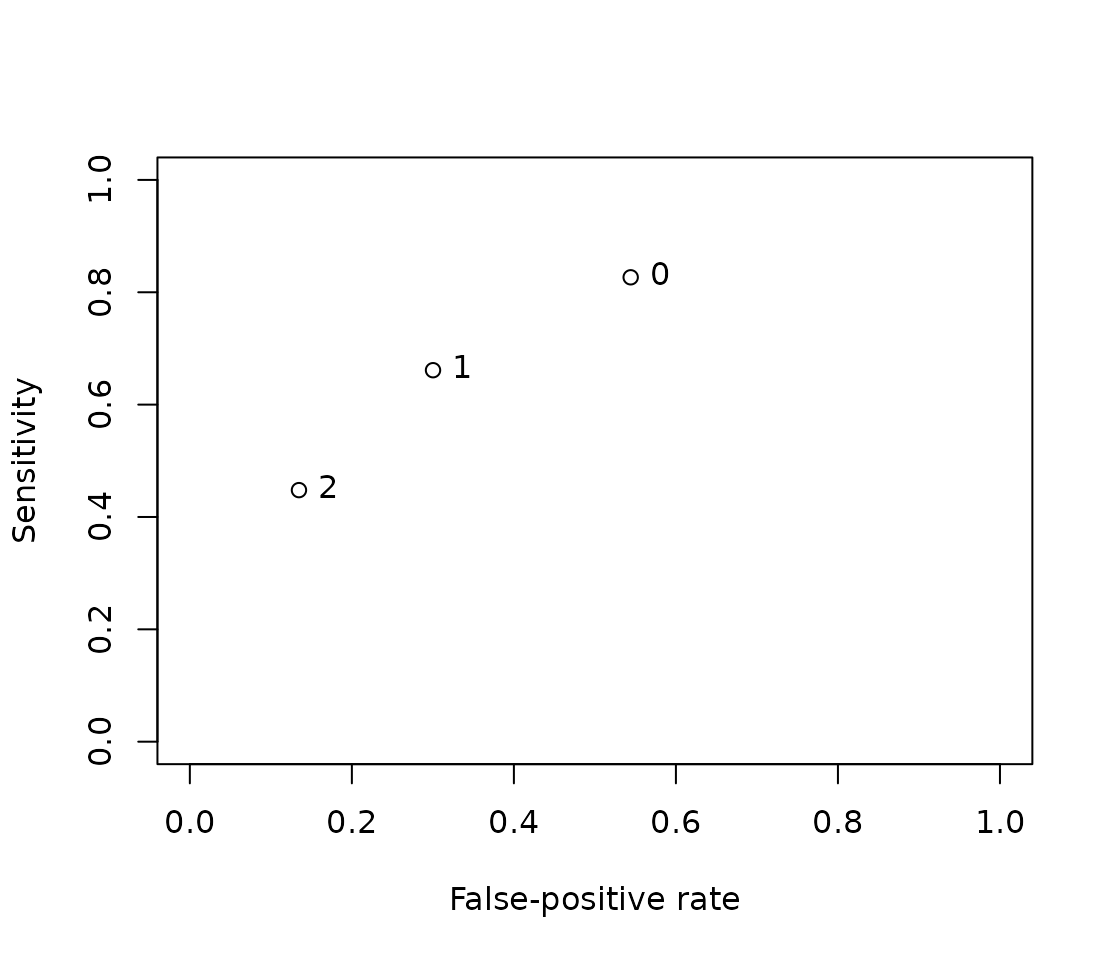
The plot shows one point per measured cutoff. These pooled means are
estimated separately and can be nonmonotone. Use the earlier
dta_sroc() example for a latent-threshold curve from a
bivariate fit. The default structure = "DIAG1" allows
different between-study variances by endpoint and cutoff, while using
the full nested sampling covariance within studies.
Fit the multinomial model to sparse threshold data
The multinomial model uses a logistic score distribution in each reference-standard stratum. It estimates separate scales and allows the two study-level locations to covary. Evaluating the distributions at their mean locations gives monotone predictions across cutoffs.
Here we reduce the fictional study sizes and set the false-positive
count at the highest cutoff to zero in study s01. The
Gaussian fit uses a continuity correction for its logits. The
multinomial fit uses the original counts, including the empty top score
bin.
sparse_thresholds <- transform(
  threshold_studies, TP = round(TP / 5), FN = 40 - round(TP / 5),
  FP = round(FP / 5), TN = 40 - round(FP / 5)
)
at_top <- sparse_thresholds$study_id == "s01" & sparse_thresholds$threshold == 2
sparse_thresholds[at_top, c("FP", "TN")] <- c(0, 40)

gaussian_sparse <- mars_dta_thresholds(sparse_thresholds, zero_cell = "add_half")
## Warning in return_estimates(q_f = q_f, q_r = q_r, estimated_pars =
## optim_values[["par"]], : Hessian inversion failed: Hessian is not positive
## definite.
multinomial_sparse <- mars_dta_thresholds(sparse_thresholds, family = "multinomial")
summary(gaussian_sparse)$pooled[c("threshold", "endpoint", "estimate")]
## threshold endpoint estimate
## 1 0 sensitivity 0.8156835
## 2 0 specificity 0.4576568
## 3 1 sensitivity 0.6563675
## 4 1 specificity 0.6934398
## 5 2 sensitivity 0.4577650
## 6 2 specificity 0.8636744## threshold endpoint estimate
## 1 0 sensitivity 0.8292480
## 2 0 specificity 0.4555459
## 3 1 sensitivity 0.6680878
## 4 1 specificity 0.7064090
## 5 2 sensitivity 0.4548215
## 6 2 specificity 0.8737247
subset(multinomial_sparse$score_bins, study_id == "s01")## study_id bin lower upper diseased non_diseased diseased_added
## 1 s01 1 -Inf 0 4 15 0
## 2 s01 2 0 1 5 9 0
## 3 s01 3 1 2 9 16 0
## 4 s01 4 2 Inf 22 0 0
## non_diseased_added
## 1 0
## 2 0
## 3 0
## 4 0Use predict() at measured cutoffs or at new values. The
prediction table flags extrapolation outside the observed cutoff range.
By default, the ROC curve spans the observed range and labels the
reported cutoffs.
##   threshold    endpoint  estimate     lower     upper extrapolated
## 1       0.5 sensitivity 0.7576664 0.7174474 0.7938060        FALSE
## 2       0.5 specificity 0.5865836 0.5500274 0.6222097        FALSE
## 3       1.5 sensitivity 0.5644324 0.5160783 0.6115911        FALSE
## 4       1.5 specificity 0.8031586 0.7741137 0.8292924        FALSE
## 5       2.5 sensitivity 0.3494205 0.3022828 0.3996980         TRUE
## 6       2.5 specificity 0.9214670 0.9026022 0.9369332         TRUE
plot(multinomial_sparse)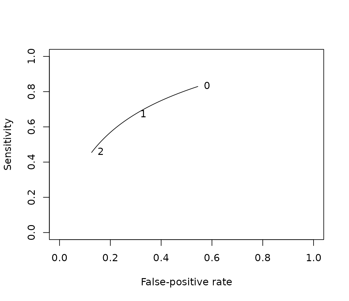
References
Reitsma, J. B., et al. (2005). Bivariate analysis of sensitivity and specificity produces informative summary measures in diagnostic reviews. Journal of Clinical Epidemiology, 58(10), 982–990. https://doi.org/10.1016/j.jclinepi.2005.02.022
Chu, H., and Cole, S. R. (2006). Bivariate meta-analysis of sensitivity and specificity with sparse data: a generalized linear mixed model approach. Journal of Clinical Epidemiology, 59(12), 1331–1332. https://doi.org/10.1016/j.jclinepi.2006.06.011
Rutter, C. M., and Gatsonis, C. A. (2001). A hierarchical regression approach to meta-analysis of diagnostic test accuracy evaluations. Statistics in Medicine, 20(19), 2865–2884. https://doi.org/10.1002/sim.942
Hamza, T. H., et al. (2009). Multivariate random effects meta-analysis of diagnostic tests with multiple thresholds. BMC Medical Research Methodology, 9, 73. https://doi.org/10.1186/1471-2288-9-73
Jones, H. E., et al. (2019). Quantifying how diagnostic test accuracy depends on threshold in a meta-analysis. Statistics in Medicine. https://doi.org/10.1002/sim.8301