
LASSO Meta-Regression with MARS
mars authors
LASSO-Meta-Regression.Rmdmars_lasso() fits sparse linear moderator models for
univariate, nested multilevel and multivariate meta-analysis. Its
wrappers are mars_lasso_univariate(),
mars_lasso_multilevel() and
mars_lasso_multivariate(). Intercepts and outcome baselines
remain unpenalized. Moderator selection is exploratory: the output
contains point estimates and numerical/tuning diagnostics, without
ordinary Wald standard errors, p-values or confidence intervals for
selected coefficients.
Equivalent Entry Points
mars(..., lasso=TRUE) calls mars_lasso()
directly and returns the same mars_lasso class. It fits one
selected penalized model, with the complete penalty path and tuning
diagnostics. Both routes share the default grid
10^seq(2,-3,length.out=20), five study-grouped folds, the
one-standard-error selection rule, unpenalized baselines and
training-fold standardization.
Pass tuning controls through lasso_args in
mars(). For example, these calls produce identical
coefficients, variance components, paths, folds, validation scores and
predictions:
controls <- list(lambda_grid=c(10,1,.1), folds=3, seed=2, selection="1se")
direct <- do.call(mars_lasso_univariate, c(list(
  data=teacher_expectancy, formula=yi~year+weeks,
  studyID="study", variance="vi"), controls))
main <- mars(teacher_expectancy, studyID="study", formula=yi~year+weeks,
  variance="vi", lasso=TRUE, lasso_args=controls)
stopifnot(identical(coef(main), coef(direct)),
  identical(main$cv, direct$cv),
  identical(predict(main), predict(direct)))
coef(main)
#> (Intercept)        year       weeks
#> 0.07774547 0.00000000 0.00000000| Setting | mars(lasso=TRUE) |
mars_lasso() |
|---|---|---|
| Input columns, formula, sampling covariance, missing handling | Ordinary top-level arguments | Same arguments |
| Penalty grid, selection, standardization, covariance estimation, correlation scale, seed | lasso_args |
Direct arguments |
| Cross-validation folds |
lasso_args$folds or
lasso_args$K
|
folds |
| Numerical convergence tolerance |
lasso_args$tol or explicit top-level
tol
|
tol |
| Fixed penalty | lasso_args=list(selection="fixed",lambda=.1) |
selection="fixed",lambda=.1 |
| Formula model structure | Omitted means univariate; "multilevel" for
nested effects |
Same |
| Multivariate structure | Omitted, "multivariate" or
"DIAG1"
|
"multivariate", inferred from effect-size
inputs |
Both routes use penalized ML. In mars(), an omitted
estimation_method uses ML for LASSO; explicitly supplied
"REML" is rejected. The multivariate LASSO model estimates
diagonal heterogeneity by outcome; explicit "UN" and
"DIAG2" are rejected. Correlations default to Fisher-z
fitting with matched sampling covariance, and predictions return
correlations. Formula responses remain on the supplied scale; sampling
variances retain matching units.
scale_formula, user weights, fixed
tau2, robust-inference arguments,
intercept=TRUE and alternative optimizers are unsupported.
To fix all heterogeneity at zero, use
lasso_args=list(heterogeneity="none"). Unsupported controls
fail explicitly. All fold diagnostics are always retained;
all_lasso_metrics=FALSE and lambda_tolerance=0
are accepted as inert controls. Other values are rejected. The
min rule breaks exact ties toward the larger penalty, and
there is no smaller-penalty tolerance rule. K and
folds, or both placements of tol, must not be
supplied together.
Use summary(), coef(),
predict() and plot() on either result.
Ordinary mars inference and diagnostic methods do not apply
to selected LASSO fits. An ordinary follow-up fit requires a separate
mars(...,lasso=FALSE) call; its ordinary tests do not
account for selecting predictors from the same data.
Objective, Scale and Penalty
For G independent studies or outermost groups, the fitting criterion is
\frac{1}{2G}\sum_{g=1}^G\left\{\log|V_g|+ (y_g-X_g\beta)^\top V_g^{-1}(y_g-X_g\beta)\right\} +\lambda\sum_j a_j|\beta_j|.
V_g includes known/estimated
sampling covariance and nonnegative variance components. The Gaussian
normalizing constant does not affect fitting and is omitted from this
objective. Cross-validation scores include that constant. a_j is zero for baselines and one for
moderators by default. Named penalty_factor values can
change moderator weights or keep specified moderators unpenalized. The
factors are not rescaled. This definition makes lambda values specific
to this objective, design and response scale; they are not numerically
interchangeable with penalties from differently normalized software.
With standardize=TRUE, each nonbaseline model-matrix
column is centered and scaled using training sample means and sample
standard deviations. If a formula explicitly omits an intercept,
predictors are scaled without centering. Encoded categorical contrasts
and interactions are penalized individually; this is not group LASSO,
and reference-level coding can affect selection. Transformed predictors
retain their specified units when coefficients are restored.
Coordinate descent updates the mean model conditional on covariance.
Bounded ML optimization updates variance components. Paths use
descending penalties, warm starts and deterministic zero-variance and
positive-variance restarts. The joint problem is nonconvex when variance
components are estimated; convergence and stationarity checks do not
establish a global optimum. heterogeneity="none" fixes
those components at zero and yields a convex penalized GLS mean
problem.
Univariate Moderator Selection
fit_uni <- mars_lasso_univariate(
  teacher_expectancy, yi ~ year + weeks, "study", "vi",
  lambda_grid=c(10,1,.1,.01), folds=3, seed=1
)
summary(fit_uni)
#> MARS LASSO meta-regression
#> Structure: univariate
#> Selected lambda: 10
#> Selection: 1se
#> Fitting scale: response
#>
#> Penalized mean-model point estimates:
#>         term estimate penalized selected
#>  (Intercept)  0.07775     FALSE     TRUE
#>         year  0.00000      TRUE    FALSE
#>        weeks  0.00000      TRUE    FALSE
#>
#> Variance components (conditional ML point estimates):
#>  component variance
#>       tau2  0.01255
#>
#> Grouped cross-validation:
#>  lambda mean_nll se_nll successful_folds full_converged eligible
#>   10.00  0.25914 0.1985                3           TRUE     TRUE
#>    1.00  0.06638 0.2656                3           TRUE     TRUE
#>    0.10  0.09697 0.2419                3           TRUE     TRUE
#>    0.01  0.10201 0.2403                3           TRUE     TRUE
#>
#> Converged full-data path fits: 4 / 4
#> Successful fold/penalty fits: 12 / 12
#>
#> Selected lambda is a grid endpoint; consider expanding the penalty range.
#>
#> Penalized point estimates; ordinary Wald inference is unavailable after selection
coef(fit_uni)
#> (Intercept)        year       weeks
#>  0.07774547  0.00000000  0.00000000
coef(fit_uni, standardized=TRUE)
#> (Intercept)        year       weeks
#>  0.07774547  0.00000000  0.00000000
The intercept is retained regardless of penalty strength. Larger
penalties usually shrink more moderator coefficients to exactly zero,
although joint variance estimation can produce more complicated paths. A
zero coefficient is a result of penalized optimization, not evidence
that a population effect is zero. Univariate heterogeneity adds
independent effect-level variance. Repeated effect records share a CV
fold via studyID; dependency beyond the specified sampling
covariance needs an appropriate multilevel or multivariate model.
predict(fit_uni, teacher_expectancy[1:4,c("year","weeks")])
#>          1          2          3          4
#> 0.07774547 0.07774547 0.07774547 0.07774547
fit_uni$path_diagnostics
#>   lambda converged iterations     mean_kkt variance_kkt attempted_starts
#> 1  10.00      TRUE          3 0.0001749780 9.000514e-09                2
#> 2   1.00      TRUE          6 0.0001153715 1.358023e-05                3
#> 3   0.10      TRUE          6 0.0001484034 1.701801e-08                3
#> 4   0.01      TRUE          5 0.0001183861 2.194152e-05                3
#>   successful_starts reason
#> 1                 2
#> 2                 3
#> 3                 3
#> 4                 3
Predictions use frozen training terms, transformations and standardization. They are population mean predictions for new studies and have no post-selection prediction intervals.
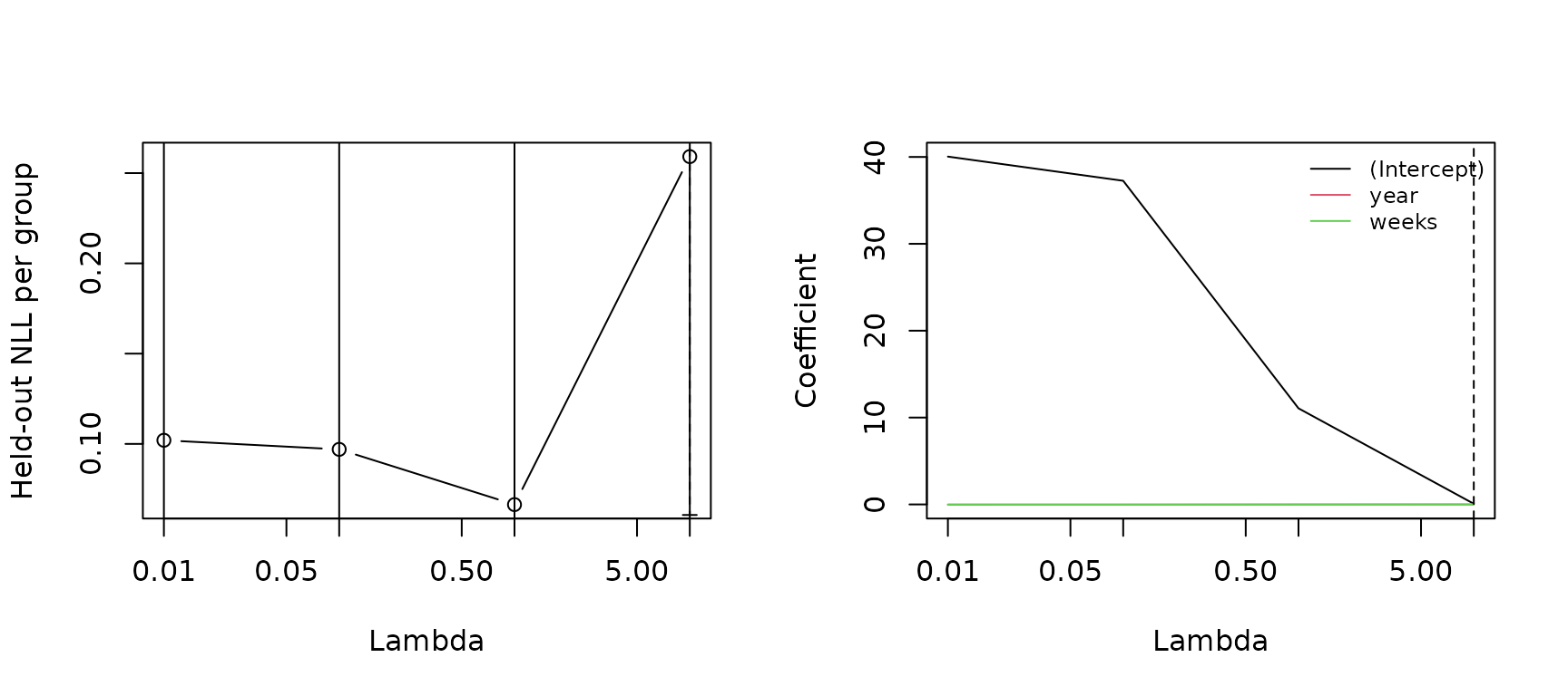
par(old_par)Grouped Cross-Validation and Selection Rules
Every study or outermost multilevel group belongs to one fold. Training-fold standardization, transformations, sampling-covariance pooling, EM moments and variance estimation are fitted without held-out observations. Known random intercept BLUPs are not used to predict the held-out group. Validation evaluates its Gaussian log density using training variance estimates and its sampling inputs. Each group contributes a complete log-density score; groups reporting more outcomes can contribute more to the score.
fit_uni$fold_assignments
#>  1 10 11 12 13 14 15 16 17 18 19  2  3  4  5  6  7  8  9
#>  1  1  1  2  1  3  2  1  3  3  2  2  2  3  3  1  3  1  2
fit_uni$cv
#>   lambda   mean_nll    se_nll successful_folds full_converged eligible
#> 1  10.00 0.25913798 0.1985097                3           TRUE     TRUE
#> 2   1.00 0.06637509 0.2655586                3           TRUE     TRUE
#> 3   0.10 0.09696911 0.2419433                3           TRUE     TRUE
#> 4   0.01 0.10200689 0.2402942                3           TRUE     TRUE
head(fit_uni$fold_scores)
#>   fold lambda group        nll
#> 1    1     10     1 -0.9887439
#> 2    1     10     6 -0.4737713
#> 3    1     10     8  1.0158657
#> 4    1     10    10  3.4299136
#> 5    1     10    11  0.8400493
#> 6    1     10    13 -0.2409988
fit_uni$fold_diagnostics
#>    fold lambda status reason
#> 1     1  10.00     ok
#> 2     1   1.00     ok
#> 3     1   0.10     ok
#> 4     1   0.01     ok
#> 5     2  10.00     ok
#> 6     2   1.00     ok
#> 7     2   0.10     ok
#> 8     2   0.01     ok
#> 9     3  10.00     ok
#> 10    3   1.00     ok
#> 11    3   0.10     ok
#> 12    3   0.01     ok
selection="min" picks the eligible penalty with the
lowest mean fold score. The default "1se" picks the largest
eligible penalty whose mean score is within one approximate standard
error of that minimum. The standard error is the standard deviation of
the K fold mean scores divided by \sqrt K. This is a tuning heuristic, not an
inferential confidence interval. Smaller Gaussian NLL is better;
negative scores are possible with concentrated densities.
Every fold must succeed, and the full-data path fit must converge, for a penalty to be eligible. Unsupported held-out factor levels or failed optimization are reported in diagnostics rather than assigned invented scores. If no penalty is eligible, fitting stops with the reasons. Expand a grid when selection reaches an endpoint. The default grid is fixed in advance; it is not learned from held-out outcomes.
The scores used to select lambda are not an independent final performance estimate. Use a separate outer grouped validation loop when tuning, selecting moderators or making predictive performance claims.
Fixed Penalty and Required Moderators
Use selection="fixed" to fit a prespecified penalty
without tuning. Named penalty weights can retain a required moderator
while penalizing others.
fit_fixed <- mars_lasso_univariate(
  teacher_expectancy, yi ~ year + weeks, "study", "vi",
  selection="fixed", lambda=.1, penalty_factor=c(year=0)
)
coef(fit_fixed)
#> (Intercept)        year       weeks
#> 40.48043990 -0.02046323 -0.01334643
fit_fixed$penalty_factor
#> (Intercept)        year       weeks
#>           0           0           1
Fixed-penalty models still undergo numerical convergence checks.
Setting lambda to zero recovers unpenalized ML/GLS point estimation when
the design and variance model are identifiable, but this interface still
returns point estimates without ordinary inference. Use the main
mars() workflow for a prespecified confirmatory model.
Refitting selected moderators on the same observations does not by
itself account for selection.
Nested Multilevel Model
fit_ml <- mars_lasso_multilevel(
  school, effect ~ year + (1 | district/study), "district", "var",
  lambda_grid=c(1,.1,.01), folds=3, seed=2
)
summary(fit_ml)
#> MARS LASSO meta-regression
#> Structure: multilevel
#> Selected lambda: 1
#> Selection: 1se
#> Fitting scale: response
#>
#> Penalized mean-model point estimates:
#>         term estimate penalized selected
#>  (Intercept)   0.1845     FALSE     TRUE
#>         year   0.0000      TRUE    FALSE
#>
#> Variance components (conditional ML point estimates):
#>  component variance
#>   district  0.05774
#>      study  0.03286
#>
#> Grouped cross-validation:
#>  lambda mean_nll se_nll successful_folds full_converged eligible
#>    1.00    1.471 0.7458                3           TRUE     TRUE
#>    0.10    1.534 0.7314                3           TRUE     TRUE
#>    0.01    1.554 0.7272                3           TRUE     TRUE
#>
#> Converged full-data path fits: 3 / 3
#> Successful fold/penalty fits: 9 / 9
#>
#> Selected lambda is a grid endpoint; consider expanding the penalty range.
#>
#> Penalized point estimates; ordinary Wald inference is unavailable after selection
predict(fit_ml,school[1:4,"year",drop=FALSE])
#>         1         2         3         4
#> 0.1844554 0.1844554 0.1844554 0.1844554
studyID names the outermost independent group, here
district. All nested studies in a district stay together in
cross-validation. Nested child labels are combined with ancestor IDs, so
reused child labels in different districts remain distinct. One additive
nested random-intercept term is supported. Random slopes, crossed terms
and variance scale formulas are not supported by this interface.
Variance components are nonnegative conditional ML point estimates under
the penalized mean model. They are unpenalized but may change as the
mean model shrinks.
Multivariate Correlations
Wide correlation inputs use a complete set of pair-named columns. Sampling covariance is retained across the correlations from each study.
set.seed(11)
cor_data <- data.frame(
  id=1:18, N=120,
  b_a=seq(.1,.35,length.out=18)+rnorm(18,sd=.005),
  c_a=seq(.2,.4,length.out=18)+rnorm(18,sd=.005),
  c_b=seq(.3,.5,length.out=18)+rnorm(18,sd=.005),
  z=seq(-1,1,length.out=18)
)
fit_cor <- mars_lasso_multivariate(
  cor_data,"id","cor",sample_size="N",variable_names=c("b_a","c_a","c_b"),
  multivariate_covs=~z,lambda_grid=c(1,.1,.01),folds=3,seed=3
)
summary(fit_cor)
#> MARS LASSO meta-regression
#> Structure: multivariate
#> Selected lambda: 1
#> Selection: 1se
#> Fitting scale: fisher_z
#>
#> Penalized mean-model point estimates:
#>       term estimate penalized selected
#>  outcome_1   0.2278     FALSE     TRUE
#>  outcome_2   0.3087     FALSE     TRUE
#>  outcome_3   0.4250     FALSE     TRUE
#>          z   0.1127      TRUE     TRUE
#>
#> Variance components (conditional ML point estimates):
#>  component variance
#>  outcome_1        0
#>  outcome_2        0
#>  outcome_3        0
#>
#> Grouped cross-validation:
#>  lambda mean_nll   se_nll successful_folds full_converged eligible
#>    1.00   -4.513 0.009122                3           TRUE     TRUE
#>    0.10   -4.516 0.007894                3           TRUE     TRUE
#>    0.01   -4.516 0.007815                3           TRUE     TRUE
#>
#> Converged full-data path fits: 3 / 3
#> Successful fold/penalty fits: 9 / 9
#>
#> Selected lambda is a grid endpoint; consider expanding the penalty range.
#>
#> Penalized point estimates; ordinary Wald inference is unavailable after selection
The default mean model has an unpenalized baseline for each outcome
and common moderator slopes across outcomes.
outcome_specific=TRUE fits separate penalized moderator
slopes for each outcome. Between-study heterogeneity is diagonal by
outcome; the sampling covariance remains fully represented. This model
does not estimate an unstructured between-outcome heterogeneity
matrix.
Correlations are fitted on the Fisher-z scale by default: z=\operatorname{atanh}(r) with delta
covariance J S J^\top, J_{ii}=1/(1-r_i^2). Coefficients are working-
scale location coefficients; prediction returns \tanh(\widehat z) rather than an expectation
integrated over random effects. prediction_scale="raw"
instead fits raw correlations and can extrapolate outside [-1,1].
For pooled covariance types, CV uses the training Olkin-Siotani numerator at each held-out sample size. Fisher-z derivatives for these held-out blocks use training pooled correlations. Simple study-specific covariance uses the supplied held-out study’s sampling inputs; those are not used to estimate training parameters.
first <- fit_cor$data[fit_cor$data$study==fit_cor$data$study[1],,drop=FALSE]
predict(fit_cor,first,type="working")
#>         1         2         3
#> 0.1150729 0.1960086 0.3123086
matrices <- predict(fit_cor,first,type="matrix",matrix_action="error")
matrices[[1]]
#>           a         b         c
#> a 1.0000000 0.1145676 0.1935364
#> b 0.1145676 1.0000000 0.3025359
#> c 0.1935364 0.3025359 1.0000000
attr(matrices,"diagnostics")
#>   group valid_before min_eigenvalue_before repaired max_abs_change
#> 1     1         TRUE             0.6844073    FALSE              0
#>   min_eigenvalue_after
#> 1            0.6844073
Matrix prediction needs the internal group and effect columns named
by study_id and effect_id. Pairwise Fisher-z
bounds do not guarantee a valid joint matrix.
matrix_action="warn" checks complete matrices;
"error" rejects invalid ones; explicit
"repair" applies the already imported Matrix package’s
nearest correlation-matrix projection and records the changes. Repair
changes estimates and supplies no inferential correction.
Long-Form Multivariate SMDs
For SMDs, supply a unique effect ID per study and a supported sampling-covariance type. Shared-control sampling covariance and diagonal outcome-specific heterogeneity are different components of the model.
smd_example <- data.frame(
  id=rep(1:15,each=2), pair=rep(c("a","b"),15), N=100,nt=50,nc=50,
  control_id="control", z=rep(seq(-1,1,length.out=15),each=2)
)
smd_example$yi <- rep(c(.1,.3),15)+.2*smd_example$z+.04*sin(1:30)
fit_smd <- mars_lasso_multivariate(
  smd_example,"id","smd",effectID="pair",sample_size="N",effectsize_name="yi",
  varcov_type="smd_shared_control",multivariate_covs=~z,
  lambda_grid=c(1,.1,.01),folds=3,seed=4
)
coef(fit_smd)
#> outcome_a outcome_b         z
#> 0.1012761 0.2992363 0.1889126
Missingness, Identification and Interpretation
missing="remove" removes incomplete required records and
leaves unrelated columns alone. For wide correlations it removes the
whole incomplete matrix. missing="em" supports continuous
moderator completion, fitted in each training fold and transferred
through frozen conditional-normal moments. Missing categorical variables
and entirely missing moderator columns are unsupported; imputation
uncertainty is not propagated.
Penalized models can have more predictors than observations, but unpenalized columns must be identifiable. Rank deficiency among penalized columns can make individual coefficients nonunique, so the output records a note. Unknown factor levels, outcome IDs and invalid covariance are explicit errors. Always inspect path and fold diagnostics before interpreting selected variables.
The fixed-covariance mean problem follows Gaussian LASSO coordinate descent; the glmnet methods paper describes this general approach. Unpenalized variance-model checks can be compared with the corresponding ML models in metafor. Neither package is a runtime dependency of this implementation. Selecting moderators and then reporting conventional p-values from a same-data refit is not selection-aware inference.