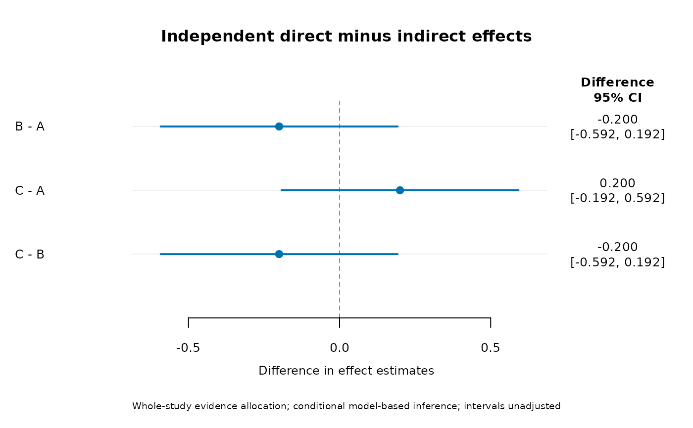
Plot covariance-aware network incoherence assessments
network_incoherence_plot.RdDisplay descriptive differences, independent node-splitting intervals, or model-based incoherence-test p-values with their calculation labelled.
Arguments
- object
A fitted joint network model.
- display
differencefor descriptive conditional differences,testsfor global/local tests, ornodesplitfor independent study-allocation splits.- method
conditionalorMLfor tests/node-splitting, orwaldfor the refitted REML design-by-treatment test display. Test displays default towald; other displays default toconditional. Descriptive differences requireconditional.- strata
Named outcome/time values selecting displayed difference or node-splitting rows. Test displays assess the full model and reject selection.
- ci_level
Confidence level for descriptive or node-splitting intervals; it does not change test p-values.
- main
Optional plot title.
- adjust
Local test or node-split multiplicity adjustment:
none,holm, orbonferroni. Difference displays requirenone. Intervals stay pointwise.- estimable_only
Logical; for
display="nodesplit", omit unavailable splits from the figure (defaultFALSE). All computed rows and the original multiplicity family are retained in the invisible return value.- point_cex
Scaling for point markers.
- label_cex
Scaling for treatment/axis labels. Font family and style inherit base graphics settings such as
par(family="sans", font=1).
Value
Invisibly returns the displayed data. difference returns a table of
differences, limits and SEs; nodesplit returns the selected full split table;
tests returns global/local test rows with a comparison label. No fit is altered.
Details
Descriptive differences. Read direct and indirect GLS summaries from
object$effects, using the original fitted total covariance. Direct evidence
uses supplied rows for the target comparison; indirect evidence removes those
rows, not whole studies. Consequently the summaries can share multi-arm study
information. The displayed difference is direct minus indirect and its SE retains
that cross-covariance. Intervals use the standard normal quantile with
heterogeneity held fixed. This is not formal independent node-splitting.
Independent splits. Call network_nodesplit() and display its
difference, lower and upper. Whole direct-evidence studies are excluded
from the indirect side. Both method choices produce normal Wald intervals;
ML changes heterogeneity estimation, not the interval into a likelihood-ratio
interval. Stratum selection occurs after calculation and does not refit a
stratum-specific model.
Test display. Call network_design_incoherence() and plot the global and
local p-values. conditional uses Wald tests with fitted covariance fixed;
ML uses refitted-ML likelihood-ratio tests. The dashed .05 line is a visual
reference, not an automatic decision rule. Local p-values use the requested
adjustment; the global p-value remains unadjusted.
For difference displays, zero denotes numerical direct/indirect agreement. Positive differences mean larger direct effects on the treatment_2-minus- treatment_1 scale; benefit direction depends on the outcome. Interpret interval width and substantive effect size. Missing evidence is labelled as unavailable; an interval containing zero or a large p-value does not establish transitivity. Diagnostics remain model-based even for a primary CR1 fit.
Examples
 d <- data.frame(study=1:9,a=rep(c("A","A","B"),3),
   b=rep(c("B","C","C"),3),effect=rep(c(.2,.6,.2),3),variance=.04)
 fit <- network_meta(d,"study","a","b","effect","variance")
 network_incoherence_plot(fit,display="nodesplit")