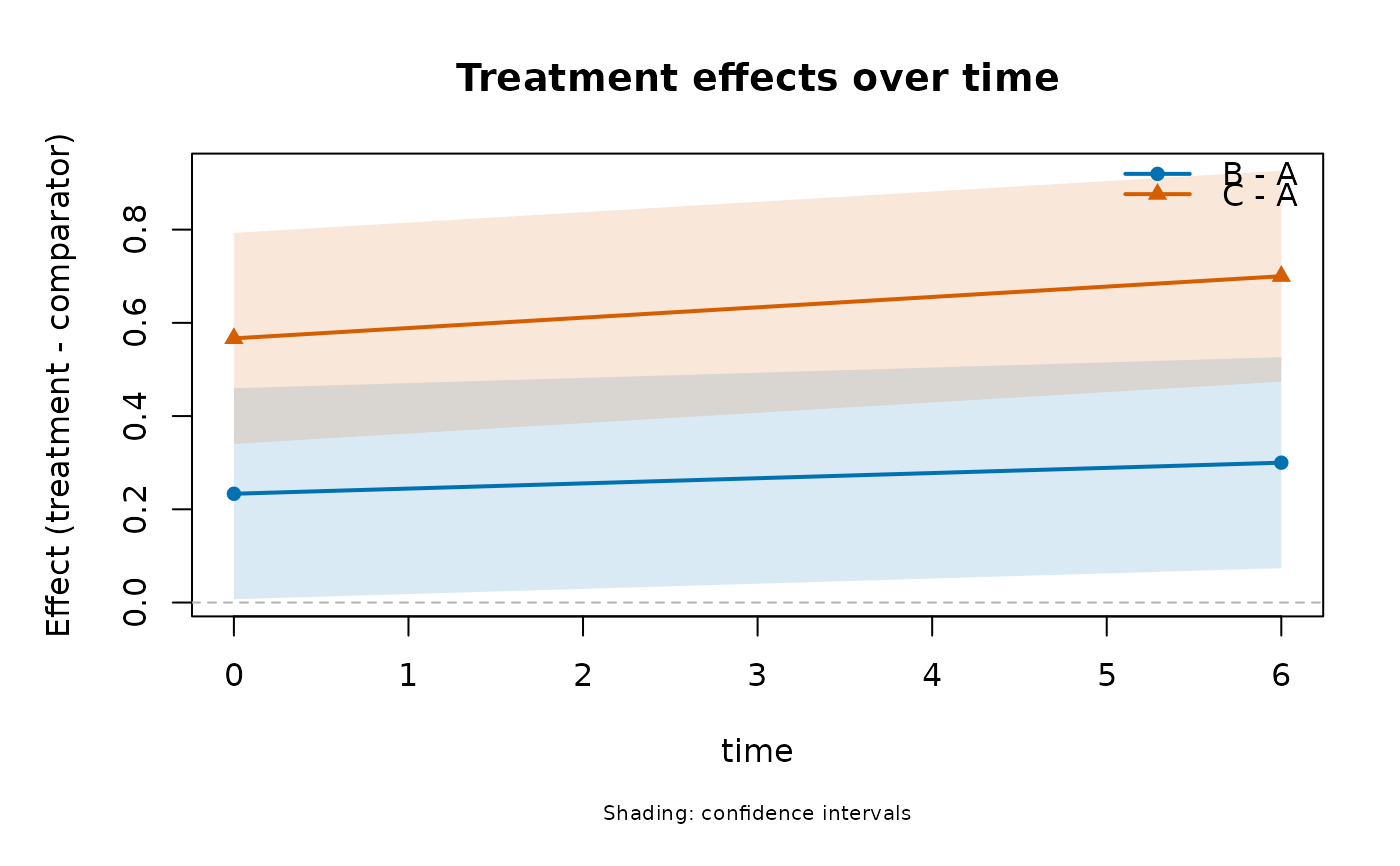
Plot network treatment effects over numeric follow-up times
network_trajectory_plot.RdPlot network treatment effects over numeric follow-up times
Usage
network_trajectory_plot(
  object,
  time,
  comparator = object$reference,
  treatments = setdiff(object$treatments, comparator),
  newdata = NULL,
  ci_level = 0.95,
  prediction = FALSE,
  benefit_direction = NULL,
  main = "Treatment effects over time",
  point_cex = 1,
  label_cex = 1
)
Arguments
- object
A one-stage coherent fit with time-specific means or a numeric time moderator.
- time
Name of the numeric time column.
- comparator
Treatment used as comparator.
- treatments
Treatments to display; defaults to all other treatments.
- newdata
Optional prediction rows containing time and all other strata and moderators. Required for fixed time trends and multiple outcomes.
- ci_level
Confidence level.
- prediction
Include dashed new-study prediction bounds.
- benefit_direction
Optional
higherorlowerinterpretation.- main
Plot title.
- point_cex
Scaling for point markers.
- label_cex
Scaling for treatment/axis labels. Font family and style inherit base graphics settings such as
par(family="sans", font=1).
Examples
dat <- data.frame(study = 1:6, a = rep(c("A", "A", "B"), 2),
                  b = rep(c("B", "C", "C"), 2),
                  yi = c(.2, .5, .3, .3, .6, .4), vi = .04)

repeated <- rbind(transform(dat, time = 0),
                  transform(dat, study = study + 6, time = 6, yi = yi + .1))
fit <- network_meta(repeated, "study", "a", "b", "yi", "vi",
                    time = "time", treatment_effects = "by_time")
network_trajectory_plot(fit, time = "time")