
Plotting network effects, evidence, and uncertainty
network-plots.RmdThe generated contrast examples below explicitly assume independent sampling errors to illustrate the display options. For studies with shared arms or repeated participants, supply their sampling covariance as shown in the main NMA vignette.
Fit a network
d <- data.frame(id=as.character(1:12),study=rep(1:6,each=2),
                a="A",b=rep(c("B","C"),6),
                g=c(.2,.5,.4,.9,-.1,.3,.7,.8,.3,.6,.1,.4),v=.04)
fit <- network_meta_coherent(d,"study","a","b","g","v",
           observation_id="id",assume_independent=TRUE,heterogeneity="common",inference="CR1")
Confidence and prediction intervals
network_forest_plot(fit,ci_level=.90,prediction=TRUE,
                    xlab="Hedges g (treatment - comparator)",
                    benefit_direction="lower")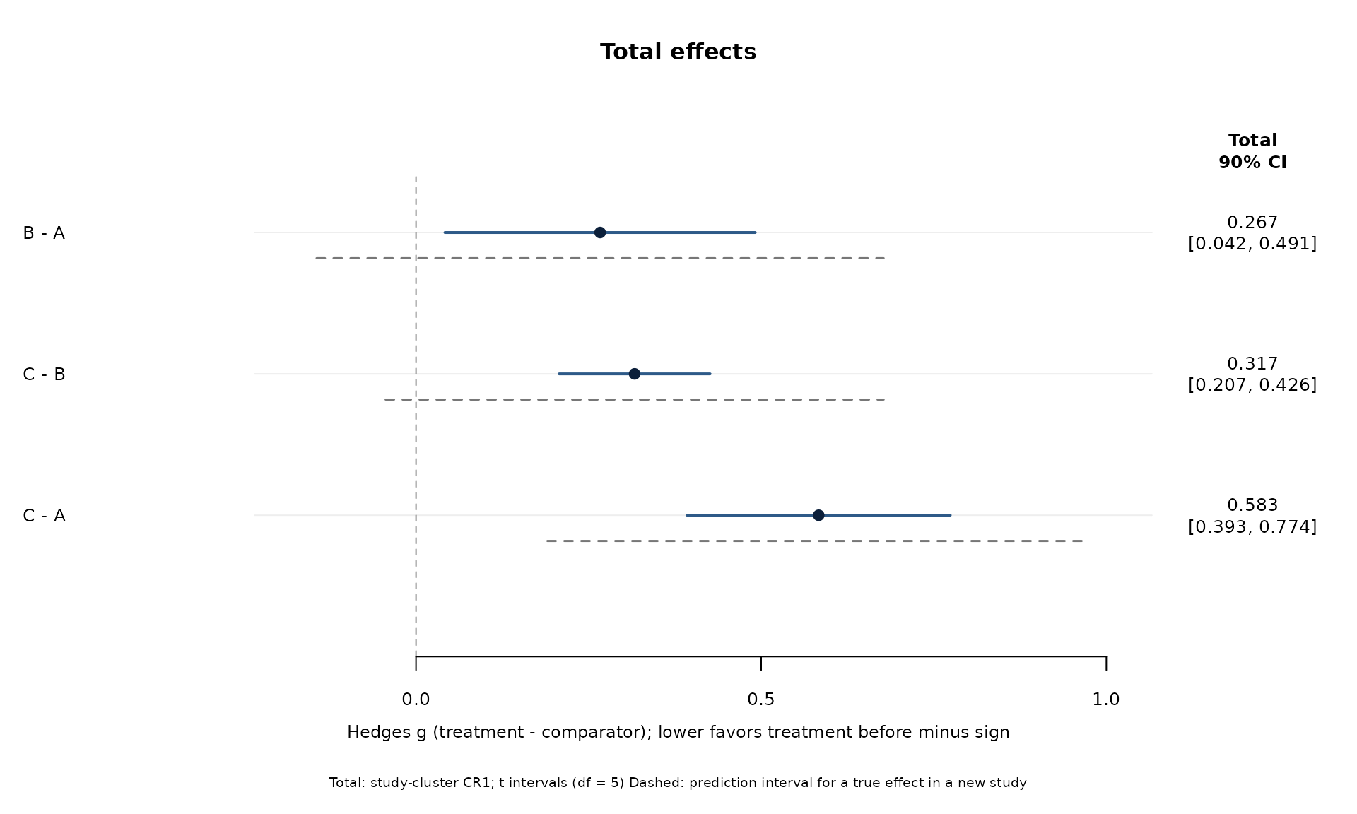
The plot recalculates intervals at the requested level. Total effects from a CR1 fit use the fitted t degrees of freedom; conditional direct and indirect summaries use their model-based normal intervals. Stored 95% intervals are not reused when 90% intervals are requested. Dashed prediction intervals describe a true contrast in a new study, rather than sampling uncertainty in a future observed SMD.
Row labels show the subtraction explicitly: B - A means
B relative to A. benefit_direction changes explanatory
text, not the sign of the fitted effects. The analyst must decide
whether higher or lower scores are preferable.
network_forest_overlay_plot(fit,ci_level=.90,prediction=TRUE,right_label="all")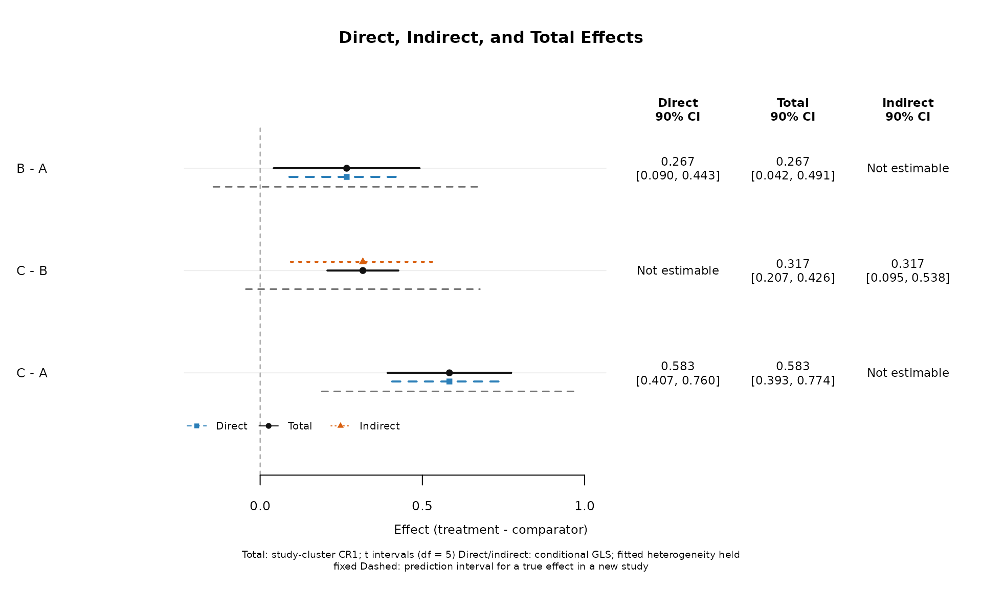
Missing direct or indirect evidence remains visible as
Not estimable. The three estimates are dependent: interval
overlap is not an incoherence test. The caption identifies conditional
versus robust inference.
Multiple outcomes and time points
d2 <- d;d2$id <- paste0(d2$id,"b");d2$g <- d2$g+.2
d$outcome <- "Depression";d2$outcome <- "Anxiety"
multiple <- network_meta_coherent(rbind(d,d2),"study","a","b","g","v",
              observation_id="id",assume_independent=TRUE,outcome="outcome",treatment_effects="by_outcome")
network_forest_plot(multiple,facet=TRUE)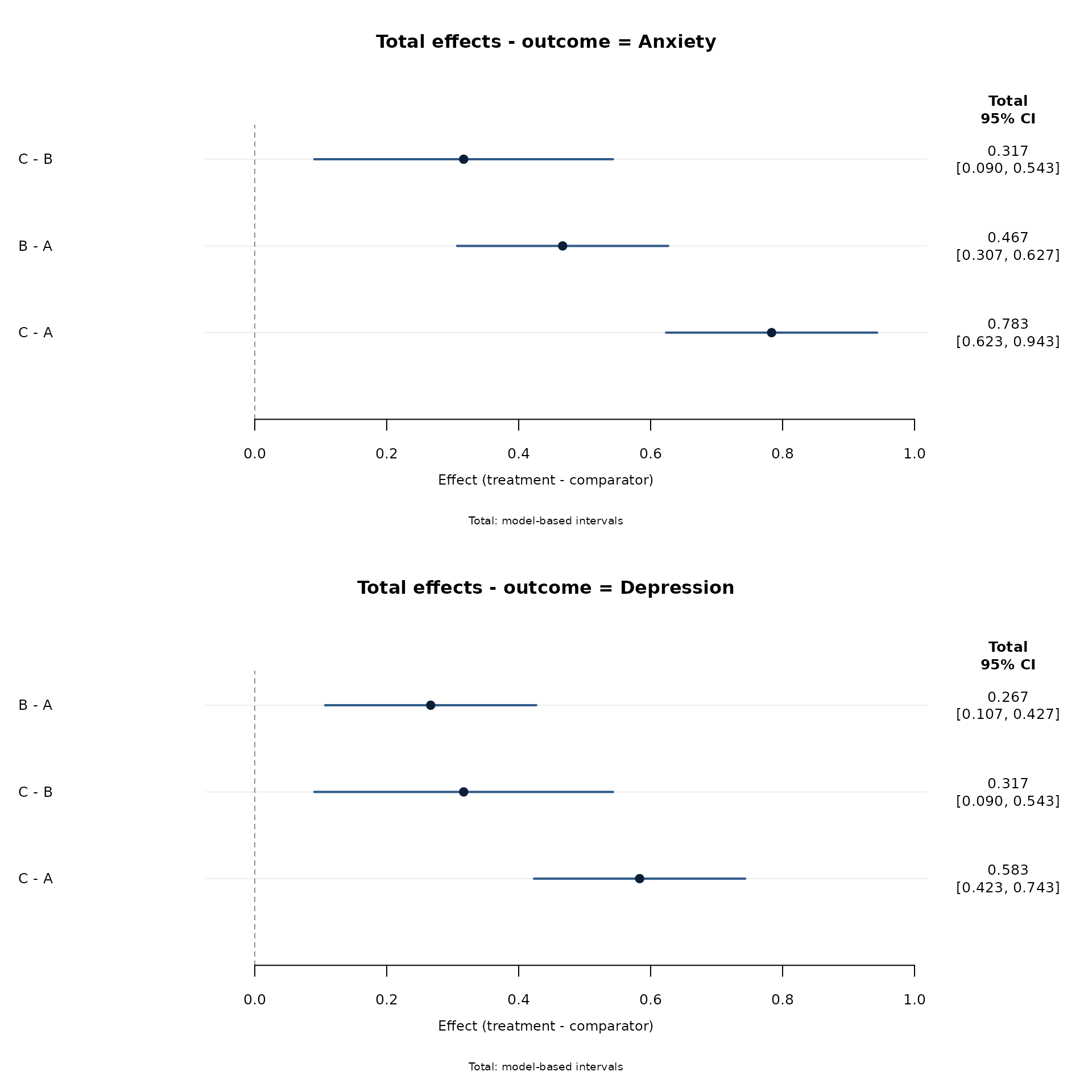
Panels share the horizontal scale. Use
strata=list(outcome="Depression") to select one outcome.
With facet=FALSE, the outcome/time combination is included
in each label. Use a taller export device for multiple panels or long
labels. These choices filter displayed estimates, without refitting the
model.
Study membership and contribution percentages
network_graph_plot(fit,show_multiarm=TRUE,edge_label=TRUE)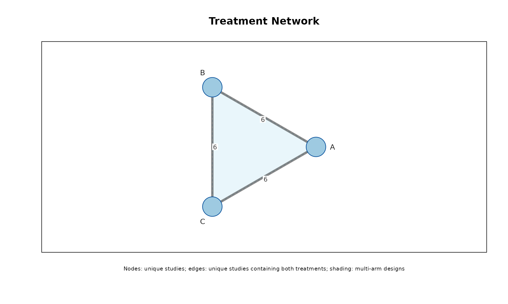
Nodes count unique studies containing a treatment, and edges count unique studies containing both treatments within a common outcome/time measurement. A multi-arm study is counted once per node and pair. A B-C edge can be supported by a study that supplied only A-B and A-C contrast rows. It does not represent an additional independent trial. Shading identifies distinct multi-arm study designs.
node_size="effects" and
edge_width="effects" explicitly count supplied contrast
rows. An implied multi-arm pair can have zero supplied rows. Selecting
outcome/time strata also filters the underlying study membership used by
the graph.
network_contribution_heatmap(fit,show_values=TRUE)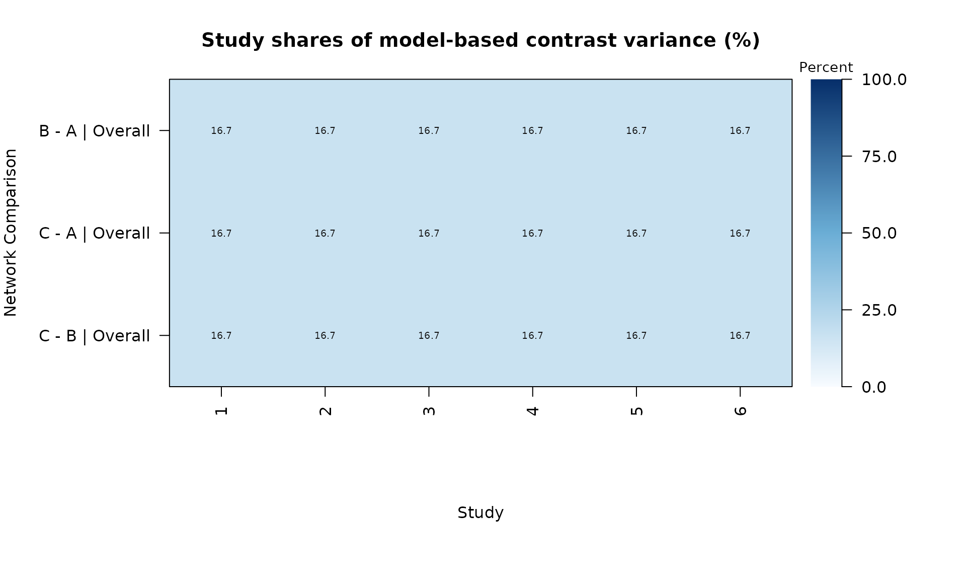
For all joint network models, columns are studies and percentages are shares of model-based contrast variance, conditional on fitted covariance. The default color scale is fixed at 0-100%, with darker colors indicating larger values. This is not a certainty-of-evidence assessment.
Incoherence displays
loop <- data.frame(id=as.character(1:30),study=1:30,
                   a=rep(c("A","A","B"),10),b=rep(c("B","C","C"),10),
                   g=rep(c(.2,.4,.8),10),v=.04)
loop_fit <- network_meta_coherent(loop,"study","a","b","g","v",observation_id="id",assume_independent=TRUE)
network_incoherence_plot(loop_fit)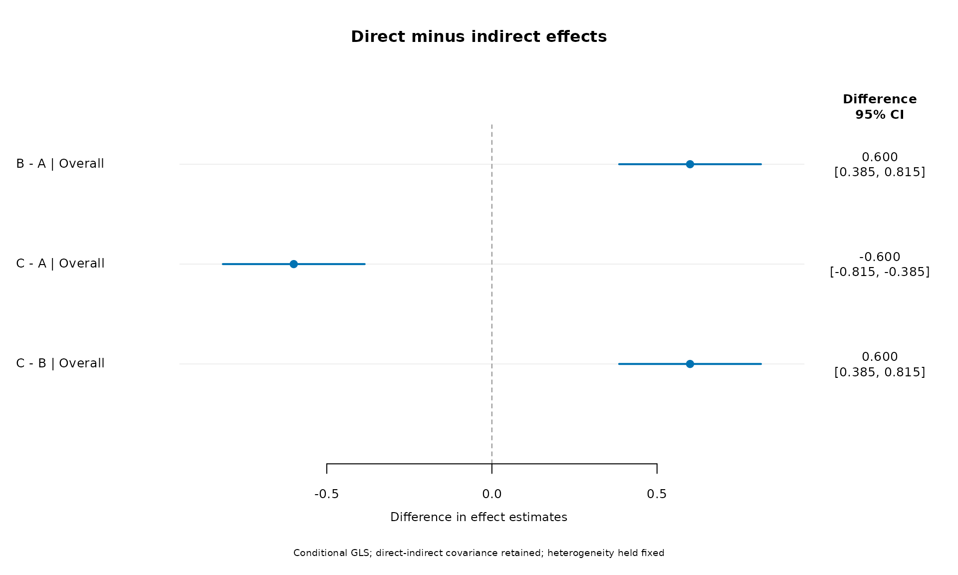
The difference interval uses the covariance between direct and
indirect estimates: its variance is
direct_se^2 + indirect_se^2 - 2 * direct_indirect_covariance.
These summaries hold heterogeneity fixed.
network_incoherence_plot(loop_fit,display="tests",method="ML")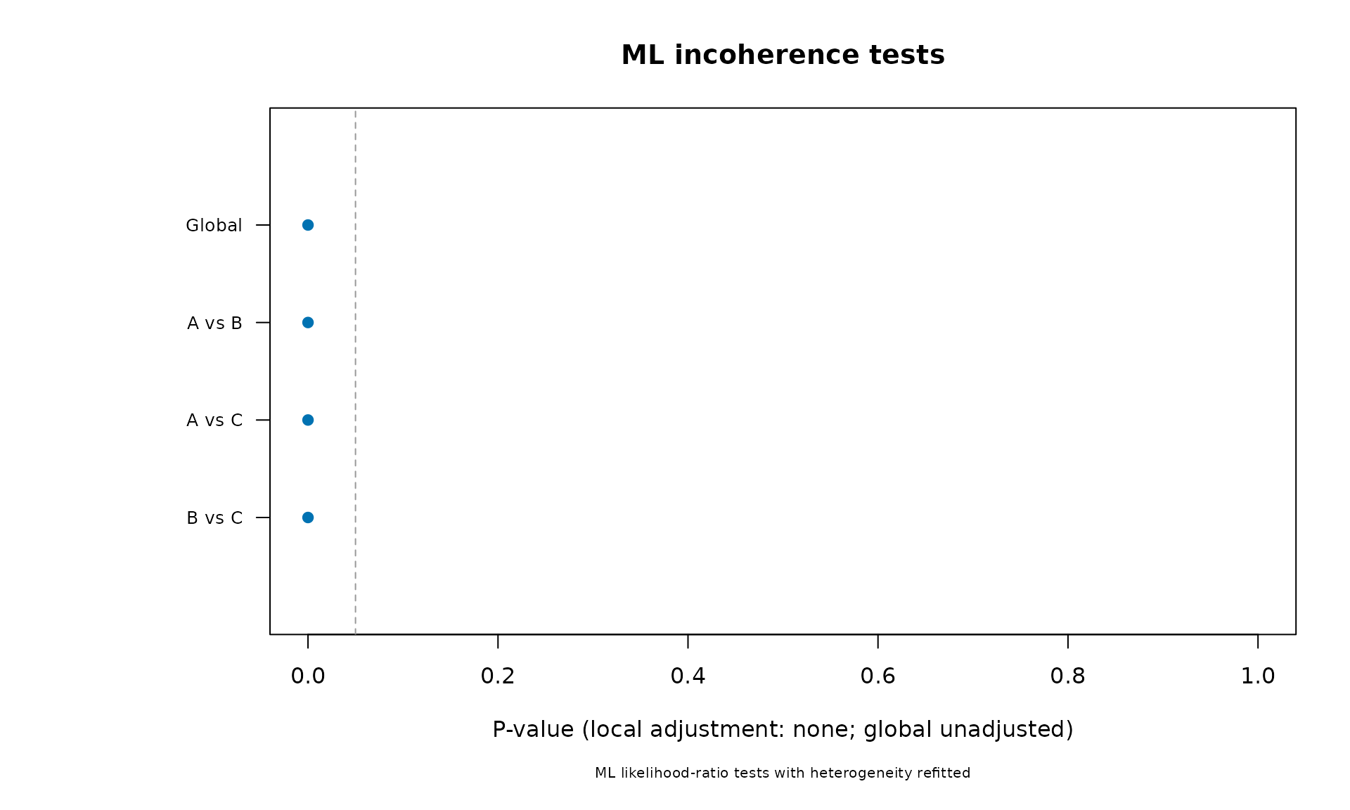
The ML display shows p-values from models that re-estimate heterogeneity under the alternative mean model. It does not label conditional difference intervals as ML intervals. Global and local tests are unadjusted for multiplicity and do not prove transitivity when nonsignificant. Test plots assess the full fitted model; they do not accept a display-only stratum subset.
Ranking uncertainty and benefit direction
network_rank_plot(fit,benefit_direction="lower",seed=12)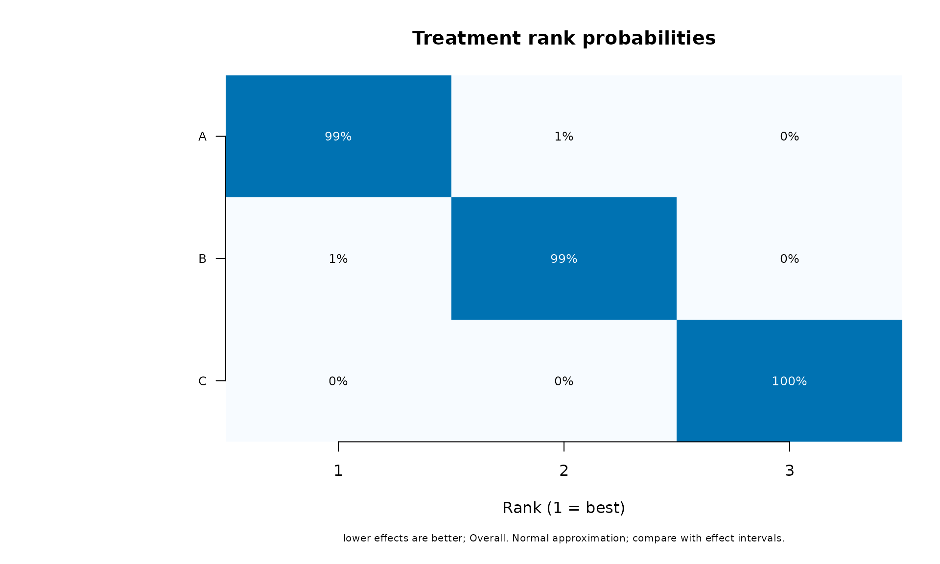
Benefit direction must be supplied explicitly. It changes the ranking calculation, not just the labels. The full rank distribution uses a multivariate normal approximation to uncertainty in the average treatment coefficients, even when the primary fit uses CR1. It is not a distribution of new-study treatment ranks. Interpret rankings alongside treatment-effect intervals. A local seed makes plots reproducible without changing the caller’s random-number state.
For multiple outcomes or times, select exactly one stratum:
network_rankings(multiple,benefit_direction="lower",strata=list(outcome="Depression"))$rankings
#>  treatment mean_effect std_error mean_rank median_rank      sucra    p_best
#>          A   0.0000000 0.0000000 1.0006000   1.0000000 99.9700000 0.9994000
#>          B   0.2666667 0.0816497 2.0019000   2.0000000 49.9050000 0.0006000
#>          C   0.5833333 0.0816497 2.9975000   3.0000000  0.1250000 0.0000000
The joint network model provides basic treatment effects relative to
a reference, with mean vector \widehat
b and covariance V_b.
network_rankings() draws b^{(s)}\sim N(\widehat b,V_b), sets the
reference-relative effect to zero, and ranks each draw. The reference
zero defines the coordinates; it does not assert that the reference
treatment’s absolute effect is known without error. An eigen-based
square root of V_b transforms
independent standard-normal noise into correlated treatment-effect
draws. Negative covariance eigenvalues are truncated to zero in this
numerical construction.
For treatment differences, preserving covariance preserves uncertainty:
\operatorname{Var}(\widehat d_i-\widehat d_j) =V_{ii}+V_{jj}-2V_{ij}.
Sampling independent treatment effects is equivalent only if it preserves the relevant contrast distribution. In the inspected netmeta 3.7.0 sampling code, independent variances are reconstructed from contrast variances; this can leave approximation errors in larger networks. The mars draws retain the fitted joint covariance instead of imposing this independent-treatment representation.
For benefit_direction="lower", the smallest draw gets
rank 1; for higher, the largest gets rank 1. Ties receive
average ranks. mean_rank and median_rank
summarize the draws, p_best and the rank-probability matrix
use the 0–1 scale, and sucra (also sucr_a)
uses the 0–100 percentage scale:
\operatorname{SUCRA}_i^{\mathrm{percent}} =100\frac{K-\overline R_i}{K-1}.
For continuous Gaussian effects and lower-is-better outcomes, the population simulation target is
\operatorname{SUCRA}_i =\frac{1}{K-1}\sum_{j\ne i} \Phi\left(\frac{\widehat d_j-\widehat d_i} {\sqrt{\operatorname{Var}(d_i-d_j)}}\right).
This fractional expected SUCRA equals the analytic Gaussian P-score
from the same contrast means and SEs. Full rank probabilities and
probability of being best involve joint events and require a compatible
joint distribution. network_rankings() currently returns
simulated SUCRA, so a fixed seed and increasing draw
counts can assess Monte Carlo stability. The following example computes
the analytic Gaussian target separately; it does not use the fit’s
multiplicity-adjusted p-values or its CR1 t p-values.
simulated <- network_rankings(fit,benefit_direction="lower",nsim=40000,seed=12)
# League entries are column-treatment minus row-treatment.
probability_better <- pnorm(fit$league_table/fit$league_table_se)
diag(probability_better) <- NA_real_
analytic_percent <- 100*rowMeans(probability_better,na.rm=TRUE)
data.frame(treatment=fit$treatments,
  simulated_SUCRA=simulated$rankings$sucra[
    match(fit$treatments,simulated$rankings$treatment)],
  analytic_Gaussian_SUCRA=analytic_percent)
#>   treatment simulated_SUCRA analytic_Gaussian_SUCRA
#> A         A        99.60875            9.957931e+01
#> B         B        50.39125            5.042069e+01
#> C         C         0.00000            1.511262e-07
CR1 fits retain their fitted sandwich covariance for the draws, while the ranking distribution remains Gaussian rather than multivariate t. All these draws condition on fitted heterogeneity and do not resample its estimation uncertainty. Effects with moderators are evaluated at moderator zero. Select one outcome/time stratum when treatment means vary across strata. Rankings describe uncertain mean effects, not new-study outcomes, clinical importance, or certainty of evidence.
The SUCRA definition follows Salanti, Ades and Ioannidis (2011), doi:10.1016/j.jclinepi.2010.03.016. The P-score connection follows Rücker and Schwarzer (2015), doi:10.1186/s12874-015-0060-8. The inspected reconstruction is in netmeta’s sampling source.
Treatment trajectories
t0 <- d[,setdiff(names(d),"outcome")];t6 <- t0
t0$time <- 0;t6$time <- 6;t6$id <- paste0(t6$id,"t6");t6$g <- t6$g-.2
time_fit <- network_meta_coherent(rbind(t0,t6),"study","a","b","g","v",
              observation_id="id",assume_independent=TRUE,time="time",treatment_effects="by_time")
network_trajectory_plot(time_fit,"time",prediction=TRUE)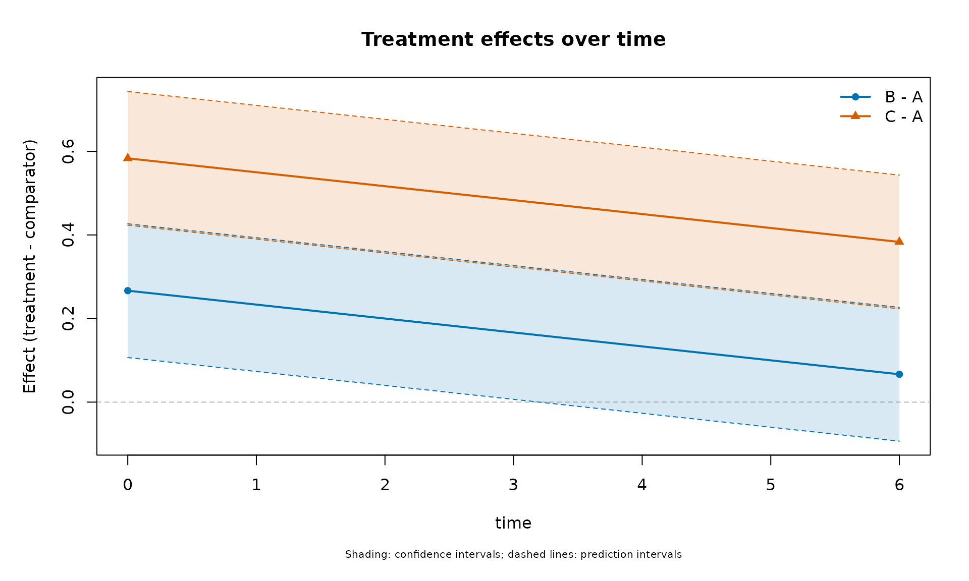
For a model with a numeric time moderator, pass newdata
containing the chosen time grid and all required moderator/stratum
columns. Supply one outcome per plot. Lines connect the specified
prediction times; they do not add an unmodelled continuous-time
assumption. Shading represents confidence intervals, while dashed bounds
represent prediction intervals.
Export
network_plot_export(
  function() network_forest_overlay_plot(fit,prediction=TRUE),
  "network-forest.pdf",width=11,height=7
)
network_plot_export(
  function() network_forest_plot(multiple,facet=TRUE),
  "network-outcomes.png",width=11,height=11,dpi=300
)
PDF and SVG exports are vector graphics; PNG uses the specified
resolution. All devices use the same requested font family
(sans by default). The helper closes its device even if
drawing fails. Plot functions return the plotted data invisibly so that
numerical values can be inspected independently of the figure.
Independent node-splitting displays
network_nodesplit(loop_fit)
#>  treatment_1 treatment_2   network network_se      prop    direct direct_se
#>            A           B 0.0000000  0.0516398 0.6666667 0.2000000 0.0632456
#>            A           C 0.6000000  0.0516398 0.6666667 0.4000000 0.0632456
#>            B           C 0.6000000  0.0516398 0.6666667 0.8000000 0.0632456
#>    indirect indirect_se direct_indirect_covariance difference        se
#>  -0.4000000   0.0894427                  0.0000000  0.6000000 0.1095445
#>   1.0000000   0.0894427                  0.0000000 -0.6000000 0.1095445
#>   0.2000000   0.0894427                  0.0000000  0.6000000 0.1095445
#>       lower      upper p_value          z direct_studies indirect_studies
#>   0.3852967  0.8147033 <0.0001  5.4772256             10               20
#>  -0.8147033 -0.3852967 <0.0001 -5.4772256             10               20
#>   0.3852967  0.8147033 <0.0001  5.4772256             10               20
#>  estimable reason      method direct_lower direct_upper indirect_lower
#>       TRUE        conditional    0.0760410    0.3239590     -0.5753045
#>       TRUE        conditional    0.2760410    0.5239590      0.8246955
#>       TRUE        conditional    0.6760410    0.9239590      0.0246955
#>  indirect_upper p_adjusted
#>      -0.2246955    <0.0001
#>       1.1753045    <0.0001
#>       0.3753045    <0.0001
network_incoherence_plot(loop_fit,display="nodesplit")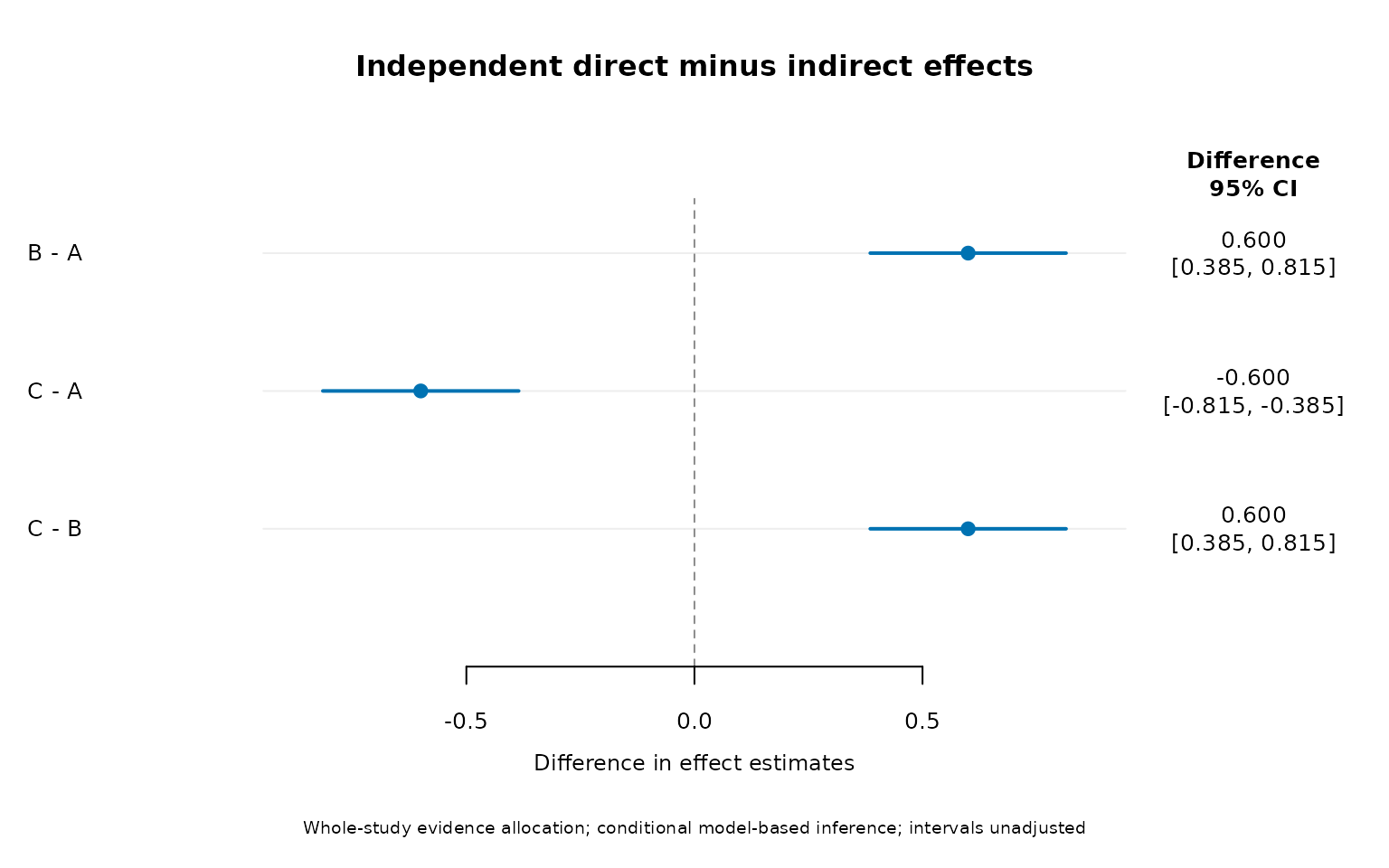
network_nodesplit_plot(loop_fit,level=.95,adjust="holm")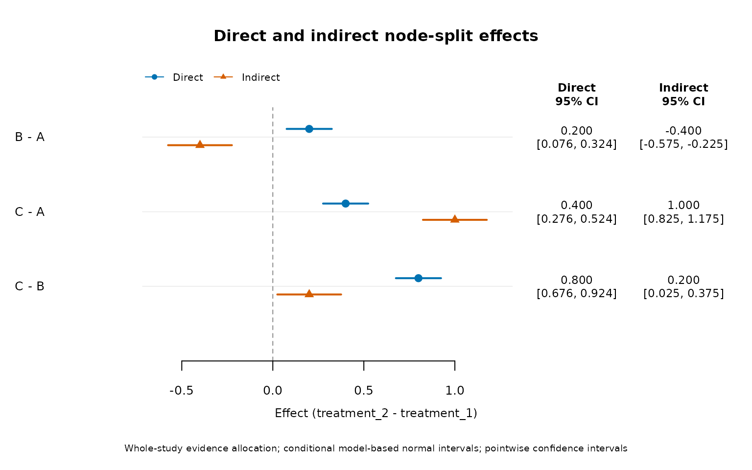
Whole direct-evidence studies are excluded from the indirect side. A network formed entirely by multi-arm studies comparing the same treatments may have no independent indirect evidence; this is reported as not estimable.