
Assessing network incoherence and transitivity
network-incoherence.RmdDistinguish the assumptions
Incoherence (called inconsistency in the cited papers) is disagreement between evidence sources beyond the model’s sampling variation and heterogeneity. Transitivity concerns comparability of effect modifiers and estimands across studies. It is assessed substantively, rather than established by a statistical test.
All three network_meta() interfaces impose coherence in
their treatment mean model. Their diagnostics share the same
implementation and retain the chosen sampling and random-treatment
covariance.
Choose the assessment
| Function | Question and computation | Interpretation |
|---|---|---|
network_transitivity() |
Deduplicated modifier distributions by observed comparison | Substantive comparability; no statistical test of transitivity |
network_design_incoherence() |
Added design-by-treatment means; refitted REML Wald, conditional Wald or refitted-ML likelihood-ratio tests | Evidence against the specified coherent mean model |
network_incoherence() |
Do direct and independent indirect effects disagree? Whole-study node splitting | Difference, interval and pair-specific Wald p-value |
network_heterogeneity() |
Do studies within the same treatment design vary? Sampling-covariance residual Q | Overall within-design Q and additive design contributions |
network_design_detachment() |
How much between-design disagreement remains after allowing each design its own effects? Studies retained; sampling-only Q | Exploratory remaining-disagreement tests, not tests of the detached design |
network_q_decomposition() |
Sampling-covariance residual Q decomposition | Additive total, within-design and between-design Q |
network_nodesplit() |
Direct study contrasts versus indirect evidence from other studies | Magnitude, direction and uncertainty of an evidence difference |
network_covariance_sensitivity() |
Refit under alternative sampling covariances | Robustness to the particular covariance assumptions chosen |
network_influence() |
Omit a study or design, refit, and compare effects | Sensitivity to evidence sources, not a study-removal rule |
network_heterogeneity_profile() |
Profile ML over one common variance | Uncertainty in heterogeneity, not an incoherence test |
summary(result, digits=3) records significant-digit
precision for printing.
print(result, digits=5, estimable_only=FALSE) can override
precision and display all hypotheses. Numeric results and adjusted
p-values retain their full precision.
network_incoherence() prints only estimable comparisons
by default. Its returned data frame retains all requested hypotheses and
nonestimability reasons. Use
print(result, estimable_only=FALSE) to inspect every row.
Display filtering does not change adjusted p-values or their family. If
none is estimable, the printout says so rather than displaying missing
comparisons.
network_incoherence() now returns the same
direct/indirect assessment as network_nodesplit(). Earlier
development calls expecting $global or $local
must use network_design_incoherence() instead, including
conditional and ML calls. Explicit
network_incoherence(method="wald") warns and returns design
tests during transition. fit$design_incoherence stores the
design test; fit$incoherence preserves that same cached
list for existing callers.
Heterogeneity concerns variation within designs; incoherence concerns evidence disagreement. NMA literature usually uses inconsistency to mean incoherence. Within-design Q uses sampling covariance alone and does not re-estimate the input model’s tau-squared.
The plot function displays the selected calculation. Its descriptive
differences can retain shared-study evidence; its nodesplit
display uses whole-study allocation.
Native diagnostic displays place the null hypothesis
(H0) after the research question. Direct–indirect tests ask
whether the difference is zero; global design tests ask whether all
identifiable design interactions are zero. Local design deviations have
their own targeted-parameter null. Within-design Q tests no residual
heterogeneity beyond sampling variation, overall and within each design.
Detachment tests no remaining between-design disagreement after relaxing
the selected design; its baseline test refers to the original network. Q
decomposition states separate null hypotheses for total, within-design
and between-design rows. I² and direct evidence proportions are
descriptive, without separate null tests.
Within-design variation and design detachment
network_heterogeneity(fit) asks how much study effects
vary within the same study design, allowing designs
separate treatment means. Its default native printout uses the heading
Within-design Q and contains overall Q and
independently testable design-specific Q, df, p-values and Q-based I²
(%). I2_percent = 100 * max(0, 1 - df/Q) for positive
independent residual df; Q at most df gives zero, and unavailable or
zero df gives NA. I² is descriptive, not a fitted variance component;
design-specific values are not additive or averaged to obtain the
overall within-design I². All designs, counts and reasons remain in
$by_design; inspect
print(result, detailed=TRUE, estimable_only=FALSE, digits=3)
for full detail. Shared moderator slopes can prevent independent
design-specific tests even when the overall residual Q is available.
network_design_detachment(fit) asks how much
between-design disagreement remains when each selected
design is allowed its own treatment effects. It retains all studies and
sampling covariance; it does not omit the selected design or refit
random-effects heterogeneity. The native display includes the baseline
sampling-only between-design Q and a four-column table of remaining Q,
df and p-value after each testable detachment. These correspond to
Q.inc.detach from netmeta::decomp.design() for
equivalent inputs and models.
A detachment p-value tests remaining disagreement, not whether the
named design is itself inconsistent. Tests overlap and are unadjusted;
changing df also changes p-values. Designs with no independent
detachment parameters, inseparable effects, or no remaining test df are
retained with status/reasons and hidden by default. Print/summary
support digits, estimable_only and
detailed, preserving all stored numerical results. These
assessments are distinct from the random-effects Higgins global test and
the pair-targeted local design-deviation tests in
network_design_incoherence().
Computational checks do not establish scientific assumptions
The fitting engine checks finite positive marginal variances, observation/covariance alignment, covariance symmetry and validity, study independence, and a nonsingular sampling contrast basis. It also checks mean-design rank and structural identifiability of estimated covariance components. Passing these checks means the specified calculation is supported, not that the chosen sampling dependence or network assumptions are scientifically correct.
Inspect fit$convergence and
fit$heterogeneity_summary. Near-zero variance or covariance
eigenvalues are flagged as boundaries; these can represent a supported
zero solution or weak information. A converged model can still contain
important evidence disagreement. Conversely, a nonestimable diagnostic
is not evidence of agreement. The assessments below address different
questions from those input checks.
A network with independent routes
d <- data.frame(study=1:18,a=rep(c("A","A","B"),6),b=rep(c("B","C","C"),6),
  effect=rep(c(.2,.8,.2),6)+rep(c(-.1,0,.1,-.05,.05,0),each=3),variance=.04,
  age=rep(c(35,55,40),6),risk=rep(c("low","high","low"),6))
fit <- network_meta(d,"study","a","b","effect","variance",heterogeneity="common")
network_transitivity(d,"study","a","b",c("age","risk"))
#>  comparison modifier        type category studies observed       mean        sd
#>      A vs B      age     numeric     <NA>       6        6 35.0000000 0.0000000
#>      A vs C      age     numeric     <NA>       6        6 55.0000000 0.0000000
#>      B vs C      age     numeric     <NA>       6        6 40.0000000 0.0000000
#>      A vs B     risk categorical      low       6        6         NA        NA
#>      A vs C     risk categorical     high       6        6         NA        NA
#>      B vs C     risk categorical      low       6        6         NA        NA
#>         min        max proportion
#>  35.0000000 35.0000000         NA
#>  55.0000000 55.0000000         NA
#>  40.0000000 40.0000000         NA
#>          NA         NA  1.0000000
#>          NA         NA  1.0000000
#>          NA         NA  1.0000000
Numeric summaries describe distributions; categorical summaries give
counts and proportions, with missing values represented separately.
Repeated identical study/comparison/modifier rows are counted once.
Differing observations remain separate, so a categorical proportion is
not necessarily a study proportion. For numeric modifiers,
observed counts finite values after deduplication and
studies includes studies with missing modifier values. SD
is the sample SD; it is unavailable with fewer than two finite values.
For categories, the denominator includes missing values and a study can
contribute more than one distinct value. An absent category is not
automatically displayed as a zero-count row. Numeric category codes
should be converted to factors before calling the function.
Compare distributions of plausible effect modifiers, rather than interpreting similar mean ages or category proportions as a validation of transitivity. These summaries do not cover unmeasured effect modifiers, and modifier imbalances alone do not establish incoherence. Implied multi-arm comparisons are not reconstructed by this descriptive helper.
Global design tests and symmetric side-splitting
network_design_incoherence(fit,method="wald",adjust="holm")
#> Higgins design-by-treatment incoherence
#> =======================================
#> Question: Do treatment effects disagree across designs after accounting for heterogeneity?
#> H0 (global): All identifiable design-by-treatment interaction parameters are zero.
#> Method: Design-by-treatment Wald tests with heterogeneity refitted by REML
#> Assumption: Asymptotic model-based tests; transitivity requires substantive assessment.
#> Null-model heterogeneity: study 0
#> Local p-value adjustment: holm (family size: 3; includes nonestimable hypotheses)
#>
#> Global test
#>  statistic df   p_value
#>  8.0000000  1 0.0046777
#>
#> Symmetric side-splitting Wald tests
#> Local coefficient covariance: GLS (conditions on fitted heterogeneity)
#> Question: Is a symmetric departure needed for each treatment pair?
#> H0 (each pair): All identifiable symmetric side-splitting gamma coefficients are zero.
#> Gamma direction: treatment 2 minus treatment 1 (see contrast).
#> Intervals: pointwise 95% normal Wald; p-value adjustment does not adjust intervals.
#> Degrees of freedom for each local test: 1
#>  comparison contrast      gamma  se_gamma   ci_lower   ci_upper statistic
#>      A vs B    B - A -0.4000000 0.1414214 -0.6771808 -0.1228192 8.0000000
#>      A vs C    C - A  0.4000000 0.1414214  0.1228192  0.6771808 8.0000000
#>      B vs C    C - B -0.4000000 0.1414214 -0.6771808 -0.1228192 8.0000000
#>    p_value p_adjusted
#>  0.0046777  0.0140332
#>  0.0046777  0.0140332
#>  0.0046777  0.0140332
#>
#> Use detailed=TRUE for variance-component and convergence details;
#> combine with estimable_only=FALSE to inspect unavailable tests and reasons.
network_design_incoherence(fit,method="conditional")
#> Higgins design-by-treatment incoherence
#> =======================================
#> Question: Do treatment effects disagree across designs after accounting for heterogeneity?
#> H0 (global): All identifiable design-by-treatment interaction parameters are zero.
#> Method: Conditional model-based Wald tests: augmented mean refits, heterogeneity held fixed
#> Assumption: Transitivity requires substantive assessment; loop closure is imposed, not tested by fitted effects.
#> Local p-value adjustment: none (family size: 3; includes nonestimable hypotheses)
#>
#> Global test
#>  statistic df   p_value
#>  8.0000000  1 0.0046777
#>
#> Symmetric side-splitting Wald tests
#> Local coefficient covariance: GLS (conditions on fitted heterogeneity)
#> Question: Is a symmetric departure needed for each treatment pair?
#> H0 (each pair): All identifiable symmetric side-splitting gamma coefficients are zero.
#> Gamma direction: treatment 2 minus treatment 1 (see contrast).
#> Intervals: pointwise 95% normal Wald; p-value adjustment does not adjust intervals.
#> Degrees of freedom for each local test: 1
#>  comparison contrast      gamma  se_gamma   ci_lower   ci_upper statistic
#>      A vs B    B - A -0.4000000 0.1414214 -0.6771808 -0.1228192 8.0000000
#>      A vs C    C - A  0.4000000 0.1414214  0.1228192  0.6771808 8.0000000
#>      B vs C    C - B -0.4000000 0.1414214 -0.6771808 -0.1228192 8.0000000
#>    p_value
#>  0.0046777
#>  0.0046777
#>  0.0046777
#>
#> Use detailed=TRUE for variance-component and convergence details;
#> combine with estimable_only=FALSE to inspect unavailable tests and reasons.
network_design_incoherence(fit,method="ML")
#> Higgins design-by-treatment incoherence
#> =======================================
#> Question: Do treatment effects disagree across designs after accounting for heterogeneity?
#> H0 (global): All identifiable design-by-treatment interaction parameters are zero.
#> Method: ML likelihood-ratio tests with heterogeneity refitted
#> Assumption: Asymptotic model-based tests; transitivity requires substantive assessment.
#> Null-model heterogeneity: study 0
#> Local p-value adjustment: none (family size: 3; includes nonestimable hypotheses)
#>
#> Global test
#>  statistic df   p_value
#>  8.0000000  1 0.0046777
#>
#> Symmetric side-splitting likelihood-ratio tests
#> Local coefficient covariance: GLS (conditions on fitted heterogeneity)
#> Question: Is a symmetric departure needed for each treatment pair?
#> H0 (each pair): All identifiable symmetric side-splitting gamma coefficients are zero.
#> Gamma direction: treatment 2 minus treatment 1 (see contrast).
#> Intervals: pointwise 95% normal Wald; p-value adjustment does not adjust intervals.
#> Degrees of freedom for each local test: 1
#>  comparison contrast      gamma  se_gamma   ci_lower   ci_upper statistic
#>      A vs B    B - A -0.4000000 0.1414214 -0.6771808 -0.1228192 8.0000000
#>      A vs C    C - A  0.4000000 0.1414214  0.1228192  0.6771808 8.0000000
#>      B vs C    C - B -0.4000000 0.1414214 -0.6771808 -0.1228192 8.0000000
#>    p_value
#>  0.0046777
#>  0.0046777
#>  0.0046777
#>
#> Use detailed=TRUE for variance-component and convergence details;
#> combine with estimable_only=FALSE to inspect unavailable tests and reasons.
network_incoherence(fit,method="conditional",adjust="holm")
#> Direct versus indirect incoherence
#> Question: Do direct and independent indirect estimates disagree for a treatment contrast?
#> H0 (each contrast): Direct and independent indirect effects are equal (difference = 0).
#> Contrast = treatment_2 - treatment_1; difference = direct - indirect.
#>
#> Method: conditional
#>
#> k = direct studies; prop = network variance / direct-only variance.
#> prop uses primary fitted model-based covariance; z = difference / SE.
#> P-value adjustment: holm; family size: 3.
#> nma = coherent estimate; diff = direct - indirect; p = raw; p_adj = adjusted.
#>
#>  contrast k      prop       nma    direct  indirect       diff          z
#>     B - A 6 0.6666667 0.3333333 0.2000000 0.6000000 -0.4000000 -2.8284271
#>     C - A 6 0.6666667 0.6666667 0.8000000 0.4000000  0.4000000  2.8284271
#>     C - B 6 0.6666667 0.3333333 0.2000000 0.6000000 -0.4000000 -2.8284271
#>          p     p_adj
#>  0.0046777 0.0140332
#>  0.0046777 0.0140332
#>  0.0046777 0.0140332
#>
#> Use detailed=TRUE for standard errors, intervals and diagnostic fields.
network_heterogeneity(fit)
#> Within-design heterogeneity
#> Question: How much do study effects vary within the same treatment design?
#> H0 (overall): No residual within-design heterogeneity beyond sampling variation.
#> Sampling covariance only.
#>
#> Overall within-design Q
#>          Q df   p_value    I2 (%)
#>  1.8750000 15 0.9999807 0.0000000
#>
#> Within-design Q
#> H0 (each design): No residual heterogeneity within the named design beyond sampling variation.
#>  design         Q df   p_value    I2 (%)
#>   A | B 0.6250000  5 0.9868300 0.0000000
#>   A | C 0.6250000  5 0.9868300 0.0000000
#>   B | C 0.6250000  5 0.9868300 0.0000000
#>
#> I2 (%) is Q-based within-design residual heterogeneity; values are not additive.
The global mean extension is design-by-treatment interaction, where a
design is the set of treatments in a study. Only independent added
parameters are tested. Local results are Symmetric
side-splitting Wald tests, following White (2015), section 3.6,
Table 1 (doi:10.1177/1536867X1501500403).
Qin et al. (2024), equation (3), describe this model and its
restrictions relative to the full design-by-treatment interaction model
(doi:10.1002/jrsm.1734).
The two target treatments are shifted symmetrically in studies
containing both, preserving multi-arm contrast identities. These
restricted augmented-mean models are not a separation into independent
direct and indirect evidence. For one estimable coefficient,
$local reports gamma, se_gamma,
ci_lower and ci_upper alongside the test
statistic. contrast gives the subtraction direction.
Intervals are pointwise 95% normal Wald intervals; Holm adjustment
applies only to p-values. $local_coefficients retains each
gamma by mean stratum for joint tests with multiple coefficients.
Coefficient covariance is the added block of the selected coefficient
covariance matrix. ML results retain likelihood-ratio test labels and
GLS Wald intervals. The default method="wald" refits the
full design-by-treatment alternative by REML and jointly Wald-tests its
identifiable incoherence coefficients, following Higgins et al. (2012)
and White et al. (2012). Heterogeneity is estimated under the
alternative, unless it was fixed. Conditional Wald tests hold fitted
covariance fixed. ML likelihood-ratio tests refit heterogeneity under
both models. REML likelihoods are not compared across different mean
designs. Output marks nonestimable tests, optimization failures, and the
fitted covariance components under ML null and alternative models.
Choosing the local coefficient covariance
# Existing default: plug-in GLS covariance, conditional on fitted heterogeneity
network_design_incoherence(fit, method="wald", local_covariance="gls")

# Stata-style covariance: retain joint mean/heterogeneity observed information
network_design_incoherence(fit, method="wald", local_covariance="observed",
adjust="none")| Option | Local coefficient covariance | Effect |
|---|---|---|
local_covariance="gls" (default) |
Inverse mean information,
(A' V^-1 A)^-1
|
Conditions on the REML heterogeneity estimate |
local_covariance="observed" |
Mean block of the inverse joint observed information in mean and heterogeneity coefficients | Includes mean/heterogeneity cross-information, reproducing White’s Stata default |
Both options use the same fitted gamma and heterogeneity. They differ
in local SEs, pointwise 95% normal confidence limits, Wald statistics
and p-values. They leave the global Higgins test unchanged.
adjust="holm" corrects the local p-values, not these
intervals. The observed calculation is asymptotic and model-based; it is
not a small-sample or robust covariance correction.
For REML, the observed option takes the Hessian of
\tfrac12\{\log|V|+(y-A\beta)^T V^{-1}(y-A\beta)+\log|A^T V^{-1}A|\}
with respect to both beta and the free variance coefficients, at their fitted values. Inverting only the mean block would recover GLS; the observed option instead inverts the joint matrix before extracting its mean block. It must not be confused with differentiating the profiled REML criterion in beta.
Use method="wald" for the observed option.
method="conditional" fixes the primary covariance, while
method="ML" reports likelihood-ratio p-values; both
explicitly reject local_covariance="observed". With fixed
tau2 or heterogeneity="none", no heterogeneity
parameters are estimated, so the two covariance options are identical.
Estimated variance boundaries, singular or non-positive-definite joint
information make the observed local test unavailable, with a reason
retained. There is no automatic GLS fallback. Inspect all rows with
print(result, detailed=TRUE, estimable_only=FALSE).
White’s smoking example (2015, p.974) supplies six symmetric
side-splitting benchmarks. With the exact counts printed on p.967,
common heterogeneity, and REML, the observed option reproduces all six
gamma estimates and SEs within 5e-7, all six three-decimal
p-values, and the explicitly printed A-C confidence interval within
1e-6. The package tests freeze those counts and references
in tests/testthat/fixtures/white2015-*; they also verify
the Hessian against finite differences, multiple variance components,
unstructured covariance, and boundary handling. Only A-C and its
reversal have confidence intervals explicitly printed; other benchmark
intervals are derived from the printed gamma and SE. These are checks
against published output, not a new Stata execution. The default GLS SEs
are up to 0.61% smaller in this example. White’s mvmeta
help describes the conditional alternative under
nouncertainv.
The conditional statistic is Q=\widehat\gamma^{T}\operatorname{Var}(\widehat\gamma)^{-1}\widehat\gamma, where gamma contains the independently added mean coefficients. The ML statistic is twice the difference between the alternative and null maximized log-likelihoods. Both use an asymptotic chi-squared reference with degrees of freedom equal to the rank increase in the mean design. The degree count is not the number of triangles visible in a network graph.
ml_tests <- network_design_incoherence(fit,method="ML")
ml_tests$global[,c("statistic","df","p_value","estimable","reason")]
#>   statistic df     p_value estimable reason
#> 1         8  1 0.004677735      TRUE
ml_tests$global[,c("null_heterogeneity","alternative_heterogeneity",
                  "null_convergence","alternative_convergence")]
#>   null_heterogeneity alternative_heterogeneity null_convergence
#> 1            study 0                   study 0                0
#>   alternative_convergence
#> 1                       0
Zero convergence codes indicate successful optimization. Covariance strings summarize variance components or the column-major entries of an unstructured basic-effect matrix; they are not intervals. Estimated heterogeneity may change when the mean is relaxed; that change alone is not a test of incoherence. If heterogeneity was fixed, ML comparisons retain its fixed value. The ML null is refitted by ML even when the primary estimate was REML.
A small p-value is evidence against the specified mean/covariance
model, not a measure of clinical importance or identification of a
uniquely problematic study. Reference distributions are asymptotic, and
local p-values are unadjusted unless adjust is specified.
Tests remain model-based for CR1 primary fits. A nonsignificant result
can reflect limited information and does not establish coherence.
Independent node-splitting
network_nodesplit(fit)
#>  treatment_1 treatment_2   network network_se      prop    direct direct_se
#>            A           B 0.3333333  0.0666667 0.6666667 0.2000000 0.0816497
#>            A           C 0.6666667  0.0666667 0.6666667 0.8000000 0.0816497
#>            B           C 0.3333333  0.0666667 0.6666667 0.2000000 0.0816497
#>   indirect indirect_se direct_indirect_covariance difference        se
#>  0.6000000   0.1154701                  0.0000000 -0.4000000 0.1414214
#>  0.4000000   0.1154701                  0.0000000  0.4000000 0.1414214
#>  0.6000000   0.1154701                  0.0000000 -0.4000000 0.1414214
#>       lower      upper   p_value          z direct_studies indirect_studies
#>  -0.6771808 -0.1228192 0.0046777 -2.8284271              6               12
#>   0.1228192  0.6771808 0.0046777  2.8284271              6               12
#>  -0.6771808 -0.1228192 0.0046777 -2.8284271              6               12
#>  estimable reason      method direct_lower direct_upper indirect_lower
#>       TRUE        conditional    0.0399696    0.3600304      0.3736829
#>       TRUE        conditional    0.6399696    0.9600304      0.1736829
#>       TRUE        conditional    0.0399696    0.3600304      0.3736829
#>  indirect_upper p_adjusted
#>       0.8263171  0.0046777
#>       0.6263171  0.0046777
#>       0.8263171  0.0046777
network_nodesplit(fit,method="ML",comparisons=data.frame(treatment_1="A",treatment_2="B"))
#>  treatment_1 treatment_2   network network_se      prop    direct direct_se
#>            A           B 0.3333333  0.0666667 0.6666667 0.2000000 0.0816497
#>   indirect indirect_se direct_indirect_covariance difference        se
#>  0.6000000   0.1154701                  0.0000000 -0.4000000 0.1414214
#>       lower      upper   p_value          z direct_studies indirect_studies
#>  -0.6771808 -0.1228192 0.0046777 -2.8284271              6               12
#>  estimable reason method direct_lower direct_upper indirect_lower
#>       TRUE            ML    0.0399696    0.3600304      0.3736829
#>  indirect_upper p_adjusted
#>       0.8263171  0.0046777
For each pair and mean stratum, a direct contrast is reconstructed
within each eligible study from its contrast basis. All direct-evidence
studies are excluded from the indirect side. This conservative
allocation preserves study independence and avoids reusing multi-arm
evidence. The fitted table gives direct and indirect effects and their
separate confidence intervals, their covariance, the difference and its
interval, counts and eligibility.
network_nodesplit_plot(fit) displays the two evidence
estimates and their intervals side by side. Conditional intervals hold
heterogeneity fixed; ML estimates it jointly in the split model.
Inference is model-based even if the primary model uses CR1. Moderators
must be constant within each direct study/stratum. Nonidentifiable
splits and covariance specifications are reported with a reason.
network_incoherence_plot(fit,display="nodesplit")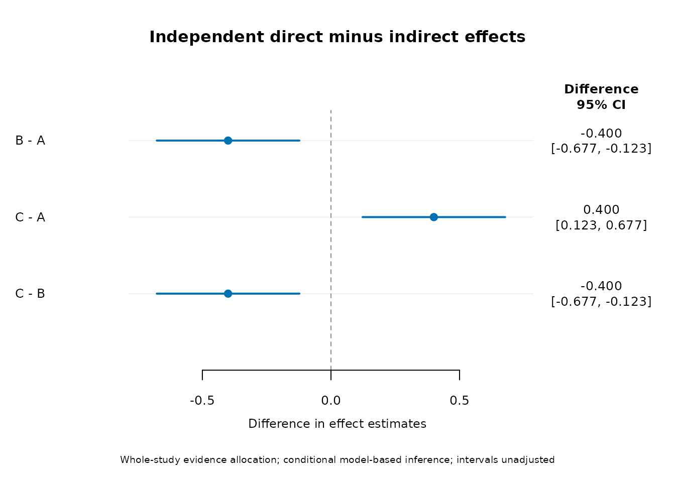
A worked interpretation on the effect scale
Use a common-effect example to make the direct/indirect calculation transparent. For A/B, direct studies estimate B minus A as .2. Independent A/C and B/C studies estimate C minus A as .6 and C minus B as .2, giving indirect B minus A of .4.
toy <- data.frame(study=1:9,a=rep(c("A","A","B"),3),
  b=rep(c("B","C","C"),3),effect=rep(c(.2,.6,.2),3),variance=.04)
toy_fit <- network_meta(toy,"study","a","b","effect","variance")
AB <- network_nodesplit(toy_fit,
  comparisons=data.frame(treatment_1="A",treatment_2="B"))
AB[,c("direct","indirect","difference","se","lower","upper","p_value")]
#>     direct  indirect difference        se      lower     upper   p_value
#>  0.2000000 0.4000000 -0.2000000 0.2000000 -0.5919928 0.1919928 0.3173105
The difference is .2 - .4 = -.2: the direct numerical effect is smaller. Its SE is .2 and the 95% interval is approximately [-.592, .192]. The interval contains zero, but also includes differences that could be important depending on the outcome. This is uncertainty about evidence agreement, not proof of agreement.
The difference variance is
\operatorname{Var}(\Delta)=\operatorname{Var}(\widehat d_D)
+\operatorname{Var}(\widehat d_I)
-2\operatorname{Cov}(\widehat d_D,\widehat d_I).
Node-splitting reports this covariance and uses a two-sided
normal Wald test in both method options. Its method="ML"
p-value is not an ML likelihood-ratio test. Normal intervals condition
on covariance estimates. For log ratios, exponentiating Delta gives a
ratio of direct to indirect ratio estimates, not a combined treatment
ratio. Whether a positive difference favors treatment B depends on
benefit direction.
direct_studies counts studies with an estimable
within-study contrast. indirect_studies counts all retained
indirect-side studies, including other strata; it is not a count of
studies on one specific indirect path. Pair selection is unordered and
does not change the returned treatment_2-minus-treatment_1
direction.
Multi-arm triangles alone cannot test agreement between independent routes
arms <- data.frame(study=rep(1:4,each=3),trt=rep(c("A","B","C"),4),
  mean=rep(c(0,.3,.6),4),sd=1,n=50)
z <- network_arm_data(arms,"study","trt",mean="mean",sd="sd")
multi <- network_meta(z$data,"study_id","treatment_1","treatment_2","effect","variance",
  observation_id="observation_id",sampling_covariance=z$sampling_covariance)
network_nodesplit(multi)
#>  treatment_1 treatment_2   network network_se      prop    direct direct_se
#>            A           B 0.3000000  0.1000000 1.0000000 0.3000000 0.1000000
#>            A           C 0.6000000  0.1000000 1.0000000 0.6000000 0.1000000
#>            B           C 0.3000000  0.1000000 1.0000000 0.3000000 0.1000000
#>  indirect indirect_se direct_indirect_covariance difference se lower upper
#>        NA          NA                         NA         NA NA    NA    NA
#>        NA          NA                         NA         NA NA    NA    NA
#>        NA          NA                         NA         NA NA    NA    NA
#>  p_value  z direct_studies indirect_studies estimable
#>       NA NA              4                0     FALSE
#>       NA NA              4                0     FALSE
#>       NA NA              4                0     FALSE
#>                                                            reason      method
#>  No independent indirect evidence after excluding direct studies. conditional
#>  No independent indirect evidence after excluding direct studies. conditional
#>  No independent indirect evidence after excluding direct studies. conditional
#>  direct_lower direct_upper indirect_lower indirect_upper p_adjusted
#>     0.1040036    0.4959964             NA             NA         NA
#>     0.4040036    0.7959964             NA             NA         NA
#>     0.1040036    0.4959964             NA             NA         NA
network_design_incoherence(multi)$global
#>   statistic df p_value estimable null_heterogeneity alternative_heterogeneity
#> 1        NA  0      NA     FALSE            study 0                      <NA>
#>   null_convergence alternative_convergence
#> 1                0                      NA
#>                                   reason
#> 1 No independent incoherence parameters.
Inspect estimable and reason before
interpreting an interval or p-value. Missing split results can arise
from unavailable independent indirect evidence, aliased mean effects,
unidentified covariance or failed optimization. A direct estimate can
still be present when an independent split is unavailable.
These studies provide direct evidence for every pair, including contrasts derived from the basis. They do not provide independent indirect evidence after study allocation. The graph’s triangle is not itself evidence of a testable incoherence loop. “Not estimable” is different from “no evidence of incoherence.”
Investigate discrepancies
network_influence(fit,unit="study")$summary
#>  omitted  unit reason max_effect_change
#>        1 study                0.0291667
#>        2 study                0.0041667
#>        3 study                0.0291667
#>        4 study                0.0166667
#>        5 study                0.0166667
#>        6 study                0.0166667
#>        7 study                0.0041667
#>        8 study                0.0291667
#>        9 study                0.0041667
#>       10 study                0.0229167
#>       11 study                0.0104167
#>       12 study                0.0229167
#>       13 study                0.0104167
#>       14 study                0.0229167
#>       15 study                0.0104167
#>       16 study                0.0166667
#>       17 study                0.0166667
#>       18 study                0.0166667
network_influence(fit,unit="design")$summary
#>  omitted   unit reason max_effect_change
#>    A | B design                0.2666667
#>    A | C design                0.2666667
#>    B | C design                0.2666667
Influence refits omit whole studies or treatment designs, rebuilding covariance and re-estimating heterogeneity unless it was fixed. For each omission, the reported maximum is \max_j\left|\widehat d_j^{(-g)}-\widehat d_j\right|, across the original reported pair/stratum estimates at the summary moderator values. It is an absolute effect change, not a standardized measure, Cook’s distance, or p-value. Changes across outcomes with different scales need separate interpretation.
The returned fits allow inspection of intervals,
heterogeneity and convergence; max_effect_change does not
summarize those quantities. Disconnected or nonidentifiable omissions
are flagged. A fitted model may be retained even if some original
prediction targets disappeared, with estimable=FALSE for
the comparison step. Such failures indicate lack of support after
omission, not necessarily incoherence. Investigate study populations,
risk of bias, effect scale and follow-up definitions; use scientifically
motivated subgroup or moderator analyses. Do not remove studies solely
because their exclusion increases a p-value.
Sensitivity to sampling covariance
The following example deliberately varies the covariance between shared-control contrasts while keeping their effects and marginal variances fixed.
shared <- data.frame(id=paste0("i",1:12),study=rep(1:6,each=2),a="A",
  b=rep(c("B","C"),6),effect=rep(c(.3,.6),6),variance=.04)
S0 <- diag(shared$variance);dimnames(S0)<-list(shared$id,shared$id)
S1 <- S0
for(ii in split(seq_len(nrow(shared)),shared$study))
  S1[ii,ii]<-matrix(c(.04,.015,.015,.04),2)
cov_fit <- network_meta(shared,"study","a","b","effect","variance",
  observation_id="id",sampling_covariance=S1)
scenarios <- network_covariance_sensitivity(cov_fit,list(independent=S0,shared_control=S1))
do.call(rbind,lapply(names(scenarios),function(name) {
  x <- scenarios[[name]]$effects
  bc <- x[x$treatment_1=="B" & x$treatment_2=="C",]
  data.frame(scenario=name,estimate=bc$total,se=bc$total_se,
    lower=bc$total_ci_lower,upper=bc$total_ci_upper)
}))
#>         scenario estimate         se      lower     upper
#> 1    independent      0.3 0.11547005 0.07368285 0.5263171
#> 2 shared_control      0.3 0.09128709 0.12108059 0.4789194
The B/C estimate is unchanged in this balanced example, while its precision changes because its variance contains the covariance term. Sensitivity can affect estimates, intervals and estimated heterogeneity in less balanced networks. A scenario must retain marginal variances, observation identities, positive-definite study covariance and study independence. Full matrices and named study-block lists are accepted. Each scenario is completely refitted; heterogeneity is re-estimated unless fixed.
The independence scenario is a deliberate perturbation for dependent data. The function does not select a correct covariance, impute participant overlap or test whether the covariance assumption holds. Use scientifically plausible scenarios and report their construction. Changing effects or standardizers requires a separate analysis rather than swapping only covariance.
Heterogeneity uncertainty is a separate question
network_heterogeneity_profile(fit)
#>       tau2     lower     upper     level
#>  0.0000000 0.0000000 0.0191341 0.9500000
#>                                                 method
#>  ML profile likelihood; approximate chi-squared cutoff
For one estimated common study variance, this function maximizes ML over treatment means at each candidate nonnegative variance, then finds an approximate likelihood- ratio interval using a one-degree-of-freedom chi-squared cutoff. It includes zero. The estimate is ML even if the primary object used REML, so the two point estimates can differ. Bounds are for variance; square-root them to express heterogeneity as an SD on the original effect scale. A wide interval signals uncertain heterogeneity, and a lower bound of zero does not establish homogeneity. Boundary/small-sample coverage is approximate. This is not an incoherence or transitivity test and is unavailable for multiple hierarchical components or unstructured covariance.
Reporting the assessment
Report the model and covariance assumptions, test method and degrees of freedom, nonestimable comparisons, direct/indirect differences with intervals, and the substantive effect-modifier assessment. Explain influential designs and plausible covariance sensitivity scenarios. Report the requested local multiplicity method and distinguish pointwise from simultaneous intervals. Extra random effects or sandwich standard errors do not repair incoherent mean assumptions. Design-specific estimates should not be automatically interpreted as a single coherent treatment ranking.
The approach follows Higgins et al. (2012), design-by-treatment incoherence, and White et al. (2012), multivariate meta-regression estimation.
Confidence intervals and multiplicity
fit_adjusted <- network_meta(d,"study","a","b","effect","variance",
  heterogeneity="common",adjust="holm")
summary(fit_adjusted)
#> Results generated with MARS: v0.6.0.8
#> Printed on: Friday, November 20, 2026
#>
#> Joint coherent network meta-analysis
#> ====================================
#>
#> Network overview
#>   Studies:                         18
#>   Pairwise comparisons:            18
#>   Treatments:                      3
#>   Designs:                         3
#>   Unique study treatment pairs:    3
#>   Modeled contrast rows:           18
#>   Pairwise comparisons count each treatment pair once per study,
#>   including implied multi-arm pairs; unique pairs are counted once overall.
#>
#> Model settings
#>   Interface:                       coherent
#>   Reference treatment:             A
#>   Effect direction:                Treatment minus A
#>   Estimation:                      REML
#>   Sampling covariance:             independent
#>   Heterogeneity structure:         common
#>   Inference:                       model
#>   Test reference distribution:     Normal (z)
#>   Convergence code:                0
#>   Covariance boundary:             TRUE
#>   Treatment p-value adjustment:    holm
#>   Adjustment family size:          3
#>
#> Residual variation (sampling covariance only)
#>        Component         Q df   p-value    I2 (%)
#>          Overall 9.8750000 16 0.8730740 0.0000000
#>   Within designs 1.8750000 15 0.9999807 0.0000000
#>  Between designs 8.0000000  1 0.0046777        NA
#>   Overall Q/I2 include within-design heterogeneity and between-design incoherence.
#>   I2 is Q-based (%); overall and within-design I2 are not additive.
#>   These are sampling-only diagnostics, separate from the random-effects Higgins test.
#>
#> Fitted variance components
#>  component      tau2
#>      study 0.0000000
#>
#> Treatment contrasts (treatment minus A; reference comparisons):
#> Raw p-values; confidence intervals: pointwise.
#>  contrast     total  total_se  statistic total_ci_lower total_ci_upper
#>     B - A 0.3333333 0.0666667  5.0000000      0.2026691      0.4639976
#>     C - A 0.6666667 0.0666667 10.0000000      0.5360024      0.7973309
#>  total_p_value total_p_adjusted
#>        <0.0001          <0.0001
#>        <0.0001          <0.0001
confint(fit_adjusted,level=.90)
#>            5%       95%
#> d_B 0.2236764 0.4429902
#> d_C 0.5570098 0.7763236
#> attr(,"level")
#> [1] 0.9
#> attr(,"adjust")
#> [1] "none"
#> attr(,"family_size")
#> [1] 2
confint(fit_adjusted,type="contrasts",adjust="bonferroni")
#>   treatment_1 treatment_2  estimate  std_error  df     lower     upper
#> 1           A           B 0.3333333 0.06666667 Inf 0.1737347 0.4929320
#> 2           A           C 0.6666667 0.06666667 Inf 0.5070680 0.8262653
#> 3           B           C 0.3333333 0.06666667 Inf 0.1737347 0.4929320
network_nodesplit(fit_adjusted,adjust="holm")
#>  treatment_1 treatment_2   network network_se      prop    direct direct_se
#>            A           B 0.3333333  0.0666667 0.6666667 0.2000000 0.0816497
#>            A           C 0.6666667  0.0666667 0.6666667 0.8000000 0.0816497
#>            B           C 0.3333333  0.0666667 0.6666667 0.2000000 0.0816497
#>   indirect indirect_se direct_indirect_covariance difference        se
#>  0.6000000   0.1154701                  0.0000000 -0.4000000 0.1414214
#>  0.4000000   0.1154701                  0.0000000  0.4000000 0.1414214
#>  0.6000000   0.1154701                  0.0000000 -0.4000000 0.1414214
#>       lower      upper   p_value          z direct_studies indirect_studies
#>  -0.6771808 -0.1228192 0.0046777 -2.8284271              6               12
#>   0.1228192  0.6771808 0.0046777  2.8284271              6               12
#>  -0.6771808 -0.1228192 0.0046777 -2.8284271              6               12
#>  estimable reason      method direct_lower direct_upper indirect_lower
#>       TRUE        conditional    0.0399696    0.3600304      0.3736829
#>       TRUE        conditional    0.6399696    0.9600304      0.1736829
#>       TRUE        conditional    0.0399696    0.3600304      0.3736829
#>  indirect_upper p_adjusted
#>       0.8263171  0.0140332
#>       0.6263171  0.0140332
#>       0.8263171  0.0140332
network_q_decomposition(fit_adjusted)
#> Network residual Q decomposition
#> Question: Does the network show residual variation within designs, between designs, or both?
#> H0 (total): Study effects follow the coherent mean model, with sampling variation only.
#> H0 (within_designs): Study effects follow the design-specific mean model, with sampling variation only.
#> H0 (between_designs): Design-specific means are compatible with a coherent network.
#> Sampling covariance only.
#>
#>        component statistic df   p_value
#>            total 9.8750000 16 0.8730740
#>   within_designs 1.8750000 15 0.9999807
#>  between_designs 8.0000000  1 0.0046777
Treatment p-value adjustment covers all unique pairs across all
reported strata. Basic coefficient tests printed by
summary() remain explicitly labelled raw; the treatment
table shows both raw and adjusted p-values. All fit intervals are
pointwise. confint(...,adjust="bonferroni") requests
simultaneous intervals across the full coefficient or treatment-contrast
family before parm selection. Holm p-value correction does
not change pointwise interval limits. CR1 coefficient and treatment
intervals use the fit’s study-count-minus-one t degrees of freedom.
Direct/indirect diagnostics remain model based.
Local design deviations and node splits have separate, explicit adjustment options. Their requested families retain nonestimable hypotheses in the size. The global test remains unadjusted. Covariance sensitivity and influence refits retain the treatment adjustment method and recalculate the family for each fit.
Local statistics and degrees of freedom must not be summed into a
heterogeneity decomposition. network_q_decomposition()
instead returns additive total, within-design and between-design
residual Q using sampling covariance alone. This differs from a
random-effects incoherence test using estimated heterogeneity.
Senn2013: comparison with netmeta
Senn2013 includes 26 studies, 10 treatments and 15 designs. This
example uses metabook::Senn2013 arm summaries for both
packages, giving 45 unique treatment pairs.
network_arm_data() retains an independent contrast basis
and its shared-arm sampling covariance. meta::pairwise()
supplies all pairwise contrasts to netmeta, which accounts for the
redundant multi-arm contrasts internally. mars effects are
treatment_2 minus treatment_1; netmeta
matrices use row minus column.
The executable comparisons require the suggested packages
metabook, meta and netmeta. If
any is unavailable, these chunks are skipped, while the code and
interpretation remain visible.
senn_arms <- metabook::Senn2013
senn_basis <- network_arm_data(senn_arms,"study","treatment",
  mean="mean",sd="sd",n="n")
senn_fit <- function(heterogeneity="common",tau2=NULL,adjust="holm") {
  network_meta(senn_basis$data,"study_id","treatment_1","treatment_2",
    "effect","variance",reference="Placebo",
    observation_id="observation_id",
    sampling_covariance=senn_basis$sampling_covariance,
    heterogeneity=heterogeneity,tau2=tau2,adjust=adjust,diagnostics=FALSE)
}
senn_common <- senn_fit("none")
senn_random <- senn_fit()
senn_pw <- meta::pairwise(treat=treatment,mean=mean,sd=sd,n=n,
  studlab=study,data=senn_arms,sm="MD")
senn_netmeta <- netmeta::netmeta(TE,seTE,treat1,treat2,studlab,
  data=senn_pw,sm="MD",reference.group="Placebo",method.tau="DL")
senn_decomp <- netmeta::decomp.design(senn_netmeta)
Sampling-covariance Q decomposition
senn_q <- network_q_decomposition(senn_random)
data.frame(component=senn_q$component,df=senn_q$df,
  mars_Q=senn_q$statistic,netmeta_Q=senn_decomp$Q.decomp$Q,
  mars_p=senn_q$p_value,netmeta_p=senn_decomp$Q.decomp$pval)
#>         component df   mars_Q netmeta_Q       mars_p    netmeta_p
#> 1           total 18 96.98407  96.98407 7.876283e-13 7.876283e-13
#> 2  within_designs 11 74.44984  74.44984 1.728088e-11 1.728088e-11
#> 3 between_designs  7 22.53422  22.53422 2.053771e-03 2.053771e-03
stopifnot(max(abs(senn_q$statistic-senn_decomp$Q.decomp$Q)) < 1e-8)
Both calculations give total Q = 96.98407 (18 df), within-design Q = 74.44984 (11 df), and between-design Q = 22.53422 (7 df, p = 0.002054). This decomposition uses sampling covariance alone, including when the supplied mars object is a random-effects fit. The existing local design-deviation tests overlap and cannot be summed to reproduce within-design Q.
The separate netmeta::Senn2013 contrast dataset rounds
standard errors to four decimal places. It produces slightly different Q
values: 96.98555, 74.45528 and 22.53027. Use the same arm-derived data
to assess numerical agreement.
Refitted Wald test and matched heterogeneity
The default mars Wald test estimates heterogeneity by REML under the
full alternative design-by-treatment model.
netmeta::decomp.design() uses a within-design
DerSimonian–Laird estimate, even when its primary network fit uses REML.
Consequently, their default random-effects diagnostic results differ
slightly.
senn_wald <- network_design_incoherence(senn_random,method="wald",adjust="holm")
tau2_dl_design <- senn_decomp$Q.inc.random$tau.within[1]^2
senn_at_dl <- network_design_incoherence(senn_fit(tau2=tau2_dl_design),method="wald")

# Full-precision alternative REML benchmark for these Senn2013 arm summaries.
# Freeze this independently checked value rather than parse the rounded
# alternative_heterogeneity display string returned by the diagnostic.
tau2_reml_design <- 0.138645507672215
senn_net_at_reml <- netmeta::decomp.design(senn_netmeta,
  tau.preset=sqrt(tau2_reml_design))$Q.inc.random.preset

data.frame(calculation=c("mars alternative REML Wald","netmeta within-design DL",
    "mars fixed at netmeta within-design DL","netmeta fixed at mars alternative REML"),
  statistic=c(senn_wald$global$statistic,senn_decomp$Q.inc.random$Q,
    senn_at_dl$global$statistic,senn_net_at_reml$Q),
  df=c(senn_wald$global$df,senn_decomp$Q.inc.random$df,
    senn_at_dl$global$df,senn_net_at_reml$df),
  p_value=c(senn_wald$global$p_value,senn_decomp$Q.inc.random$pval,
    senn_at_dl$global$p_value,senn_net_at_reml$pval),
  tau2=c(tau2_reml_design,tau2_dl_design,tau2_dl_design,tau2_reml_design))
#>                              calculation statistic df   p_value      tau2
#> 1             mars alternative REML Wald  2.274443  7 0.9431037 0.1386455
#> 2               netmeta within-design DL  2.194075  7 0.9483223 0.1442039
#> 3 mars fixed at netmeta within-design DL  2.194075  7 0.9483223 0.1442039
#> 4 netmeta fixed at mars alternative REML  2.274443  7 0.9431037 0.1386455
stopifnot(abs(senn_at_dl$global$statistic-senn_decomp$Q.inc.random$Q) < 1e-8,
  abs(senn_wald$global$statistic-senn_net_at_reml$Q) < 1e-6)
mars gives chi-squared = 2.274443, 7 df, p = 0.943104 at alternative REML tau-squared = 0.138646. netmeta gives 2.194075, 7 df, p = 0.948322 at within-design DL tau-squared = 0.144204. Matching either tau-squared value makes the statistics agree. The conditional mars test instead uses coherent-model REML tau-squared = 0.099915 and gives 3.054879, 7 df, p = 0.879879.
The small sampling-only p-value and large random-effects p-value answer different questions because their covariance assumptions differ. Neither a large p-value nor agreement between software packages establishes transitivity.
Treatment intervals and adjusted p-values
Match coherent-model heterogeneity separately from the alternative-model heterogeneity used for the global Wald diagnostic. Here netmeta is fixed at the mars coherent REML estimate. The matching comparison also checks common-effect results. All 45 unique pairs form the multiplicity family before selecting a subset for display.
senn_net_matched <- netmeta::netmeta(TE,seTE,treat1,treat2,studlab,
  data=senn_pw,sm="MD",reference.group="Placebo",
  method.tau="DL",tau.preset=sqrt(senn_random$fit$variances["study"]))
senn_comparisons <- list(
  common=list(mars=senn_common,net=senn_netmeta,type="common"),
  matched_random=list(mars=senn_random,net=senn_net_matched,type="random"))
senn_errors <- do.call(rbind,lapply(names(senn_comparisons),function(name) {
  case <- senn_comparisons[[name]]
  ci <- confint(case$mars,type="contrasts")
  simultaneous <- confint(case$mars,type="contrasts",adjust="bonferroni")
  ij <- cbind(ci$treatment_2,ci$treatment_1)
  net_est <- case$net[[paste0("TE.",case$type)]][ij]
  net_se <- case$net[[paste0("seTE.",case$type)]][ij]
  net_p <- case$net[[paste0("pval.",case$type)]][ij]
  net_lower <- case$net[[paste0("lower.",case$type)]][ij]
  net_upper <- case$net[[paste0("upper.",case$type)]][ij]
  # netmeta p-values are corrected explicitly using the same 45-pair family.
  net_holm <- p.adjust(net_p,"holm",n=45)
  net_bonferroni <- p.adjust(net_p,"bonferroni",n=45)
  mars_bonferroni <- p.adjust(case$mars$effects$total_p_value,"bonferroni",n=45)
  critical <- qnorm(1-.05/(2*45))
  data.frame(model=name,
    max_effect_difference=max(abs(ci$estimate-net_est)),
    max_pointwise_CI_difference=max(abs(c(ci$lower-net_lower,ci$upper-net_upper))),
    max_Holm_difference=max(abs(case$mars$effects$total_p_adjusted-net_holm)),
    max_Bonferroni_p_difference=max(abs(mars_bonferroni-net_bonferroni)),
    max_simultaneous_CI_difference=max(abs(c(
      simultaneous$lower-(net_est-critical*net_se),
      simultaneous$upper-(net_est+critical*net_se)))))
}))
senn_errors
#>            model max_effect_difference max_pointwise_CI_difference
#> 1         common          7.827072e-14                7.949197e-14
#> 2 matched_random          1.376677e-14                1.498801e-14
#>   max_Holm_difference max_Bonferroni_p_difference
#> 1        8.768541e-13                1.530998e-13
#> 2        3.369527e-14                3.985701e-14
#>   max_simultaneous_CI_difference
#> 1                   8.026912e-14
#> 2                   1.598721e-14
stopifnot(max(as.matrix(senn_errors[,-1])) < 1e-8)
Estimates, pointwise 95% intervals, Holm/Bonferroni p-values and Bonferroni simultaneous 95% intervals agree to numerical precision. Choosing REML in both primary packages alone does not ensure identical tau-squared estimates for this multi-arm dataset; fixing the same tau-squared isolates the treatment calculations.
senn_ci <- confint(senn_random,type="contrasts")
senn_simultaneous <- confint(senn_random,type="contrasts",adjust="bonferroni")
keep <- senn_ci$treatment_1=="Placebo" | senn_ci$treatment_2=="Placebo"
ii <- which(keep)
sign <- ifelse(senn_ci$treatment_1[ii]=="Placebo",1,-1)
data.frame(treatment=ifelse(sign==1,senn_ci$treatment_2[ii],senn_ci$treatment_1[ii]),
  estimate=sign*senn_ci$estimate[ii],
  lower=ifelse(sign==1,senn_ci$lower[ii],-senn_ci$upper[ii]),
  upper=ifelse(sign==1,senn_ci$upper[ii],-senn_ci$lower[ii]),
  p_raw=senn_random$effects$total_p_value[ii],
  p_Holm_45=senn_random$effects$total_p_adjusted[ii],
  simultaneous_lower=ifelse(sign==1,senn_simultaneous$lower[ii],-senn_simultaneous$upper[ii]),
  simultaneous_upper=ifelse(sign==1,senn_simultaneous$upper[ii],-senn_simultaneous$lower[ii]))
#>       treatment   estimate      lower       upper        p_raw    p_Holm_45
#> 1      Acarbose -0.8413643 -1.3086715 -0.37405704 4.174149e-04 1.669660e-02
#> 2    Benfluorex -0.7369003 -1.2809871 -0.19281358 7.941745e-03 3.017863e-01
#> 3     Metformin -1.1284038 -1.4212259 -0.83558179 4.259478e-14 1.874170e-12
#> 4      Miglitol -0.9498845 -1.3913730 -0.50839604 2.476174e-05 1.039993e-03
#> 5  Pioglitazone -1.1294046 -1.5447550 -0.71405416 9.850679e-08 4.235792e-06
#> 6 Rosiglitazone -1.2337387 -1.4757094 -0.99176802 1.630766e-23 7.338447e-22
#> 7   Sitagliptin -0.5700000 -1.2392244  0.09922436 9.504514e-02 1.000000e+00
#> 8  Sulfonylurea -0.4175277 -0.8734346  0.03837917 7.265845e-02 1.000000e+00
#> 9  Vildagliptin -0.7000000 -1.3678682 -0.03213179 3.995056e-02 1.000000e+00
#>   simultaneous_lower simultaneous_upper
#> 1          -1.618817        -0.06391111
#> 2          -1.642091         0.16828995
#> 3          -1.615568        -0.64123947
#> 4          -1.684383        -0.21538568
#> 5          -1.820418        -0.43839129
#> 6          -1.636302        -0.83117510
#> 7          -1.683380         0.54338017
#> 8          -1.176014         0.34095886
#> 9          -1.811124         0.41112397
For Vildagliptin minus Placebo, the pointwise interval is [-1.368, -0.032], raw p = 0.03995 and Holm-adjusted p = 1 across all 45 pairs. Its simultaneous Bonferroni interval is [-1.811, 0.411]. Adjustment over only nine Placebo comparisons defines a different family and should be labelled explicitly.
Node splitting: align evidence allocation and variance fitting
network_nodesplit() reports direct_lower,
direct_upper, indirect_lower and
indirect_upper for the separate evidence estimates. These
are pointwise normal intervals at the requested level;
lower and upper remain the limits for the
direct-minus-indirect difference. Holm adjustment applies to the
difference-test p-values and does not change these confidence intervals.
An available direct estimate and interval are retained even if an
independent indirect route is unavailable.
senn_nodes <- network_nodesplit(senn_random,adjust="holm")
senn_nodes[senn_nodes$estimable,c("treatment_1","treatment_2",
  "direct","direct_lower","direct_upper",
  "indirect","indirect_lower","indirect_upper","p_value","p_adjusted")]
#>    treatment_1   treatment_2     direct direct_lower direct_upper   indirect
#>       Acarbose     Metformin -0.2000000   -1.1358146    0.7358146 -0.3249627
#>       Acarbose       Placebo  0.8549361    0.2757129    1.4341593  0.8047267
#>       Acarbose  Sulfonylurea  0.4000000   -0.2898861    1.0898861  0.4509845
#>      Metformin  Pioglitazone  0.1600000   -0.4814651    0.8014651 -0.1284622
#>      Metformin       Placebo  1.1845579    0.7929590    1.5761568  1.0667914
#>      Metformin Rosiglitazone -0.0710538   -0.6119150    0.4698075 -0.1226901
#>      Metformin  Sulfonylurea  0.3700000   -0.2915579    1.0315579  0.9931698
#>   Pioglitazone       Placebo  1.3000000    0.6324449    1.9675551  1.0216458
#>   Pioglitazone Rosiglitazone -0.1000000   -0.8159169    0.6159169 -0.1066745
#>        Placebo Rosiglitazone -1.1794097   -1.4573460   -0.9014735 -1.4038546
#>  Rosiglitazone  Sulfonylurea  1.2000000    0.5195702    1.8804298  0.5205260
#>  indirect_lower indirect_upper   p_value p_adjusted
#>      -0.9027959      0.2528704 0.8237769  1.0000000
#>      -0.0644084      1.6738619 0.9249346  1.0000000
#>      -0.2852648      1.1872339 0.9211064  1.0000000
#>      -0.6992155      0.4422911 0.5102386  1.0000000
#>       0.6180923      1.5154904 0.6983336  1.0000000
#>      -0.5075238      0.2621436 0.8788210  1.0000000
#>       0.3911369      1.5952027 0.1721058  1.0000000
#>       0.4910913      1.5522002 0.5223033  1.0000000
#>      -0.6327572      0.4194083 0.9882519  1.0000000
#>      -1.8956697     -0.9120396 0.4361528  1.0000000
#>      -0.0767178      1.1177699 0.1413051  1.0000000
network_nodesplit_plot(senn_random,adjust="holm",
  comparisons=senn_nodes[senn_nodes$estimable,c("treatment_1","treatment_2")])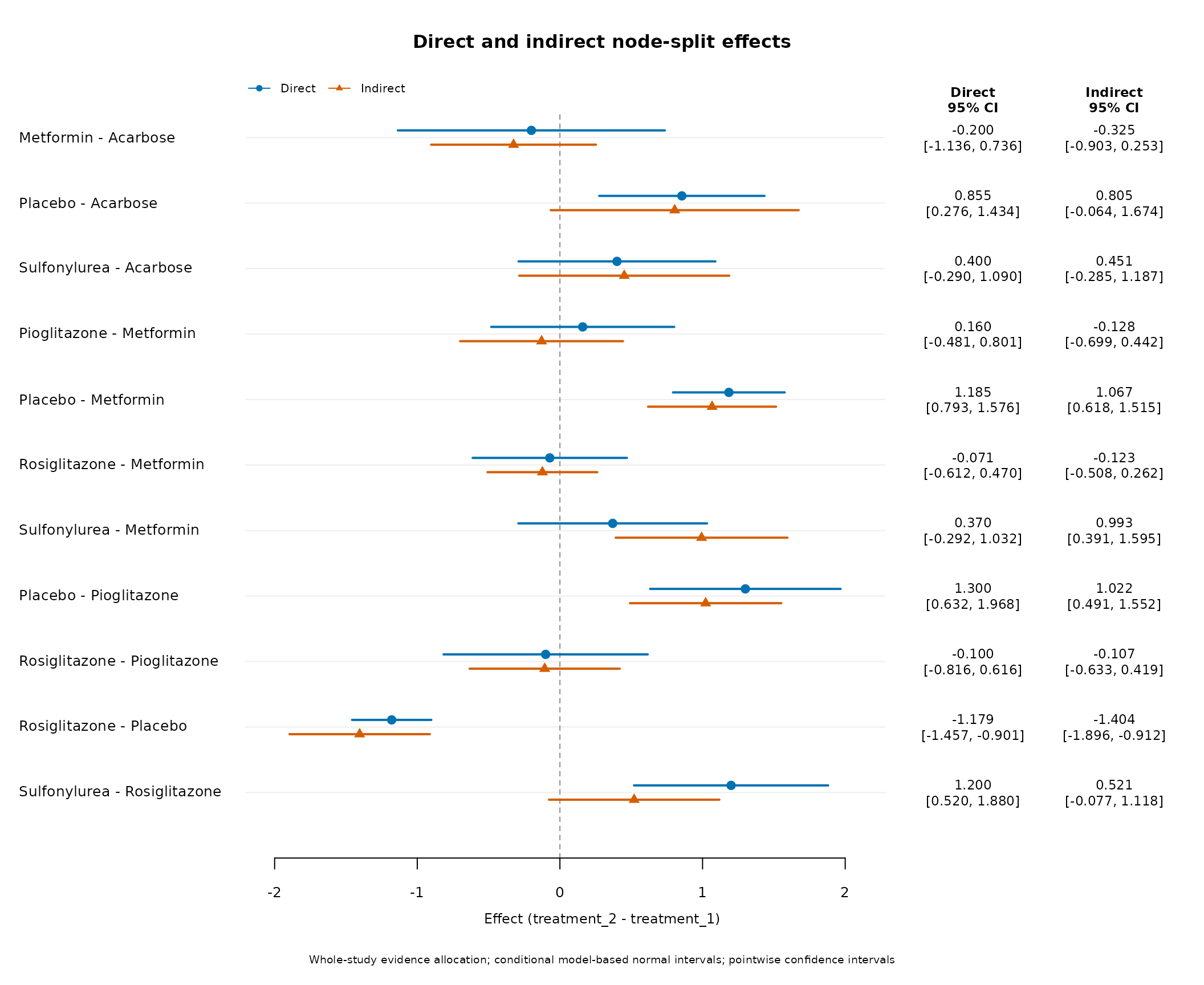
The plot places direct and indirect estimates on one effect axis with
separate symbols and numerical columns. The display above selects the 11
estimable pairs; its returned Holm values use that requested family. The
preceding table uses all 45 pairs, retaining unavailable hypotheses in
the family size. To retain that family in a plot, omit
comparisons (unavailable evidence is labelled). Confidence
interval overlap is not a test of coherence; inspect the difference
interval and its covariance-aware Wald test. Unlike
network_forest_overlay_plot(), this plot uses the
whole-study node-split allocation rather than descriptive conditional
GLS summaries.
The following comparisons were checked with netmeta 3.7.0. Matching
the primary network tau-squared does not guarantee
identical node splits. mars method="conditional" removes
whole direct-evidence studies from the indirect network and fixes their
heterogeneity. netmeta Back-calculation reuses network
estimates and direct-evidence proportions. Its SIDDE option
excludes direct design evidence, but in version 3.7.0 refits
indirect-network heterogeneity without forwarding the original tau
preset. The direct estimate still uses primary-fit heterogeneity. mars
method="ML" instead jointly refits one heterogeneity model
for its transformed direct/indirect data; it is not identical to
SIDDE.
This helper aligns netmeta’s comparison direction before displaying differences, intervals and adjusted p-values. All requested pairs form each Holm family before unavailable results or display subsets are removed.
compare_splits <- function(m,n,method="Back-calculation") {
  ms <- network_nodesplit(m,method="conditional",adjust="holm")
  ns <- netmeta::netsplit(n,method=method)$compare.random
  pairs <- strsplit(as.character(ns$comparison),":",fixed=TRUE)
  keys <- vapply(pairs,function(x)paste(sort(x),collapse=" vs "),character(1))
  ix <- match(paste(pmin(ms$treatment_1,ms$treatment_2),
    pmax(ms$treatment_1,ms$treatment_2),sep=" vs "),keys)
  sign <- vapply(seq_len(nrow(ms)),function(i) {
    if(is.na(ix[i])) NA_real_ else if(pairs[[ix[i]]][1]==ms$treatment_2[i]) 1 else -1
  },numeric(1))
  data.frame(method=method,treatment_1=ms$treatment_1,treatment_2=ms$treatment_2,
    mars_estimable=ms$estimable,mars_difference=ms$difference,
    netmeta_difference=sign*ns$TE[ix],mars_se=ms$se,netmeta_se=ns$seTE[ix],
    mars_lower=ms$lower,mars_upper=ms$upper,
    netmeta_lower=ifelse(sign==1,ns$lower[ix],-ns$upper[ix]),
    netmeta_upper=ifelse(sign==1,ns$upper[ix],-ns$lower[ix]),
    mars_Holm=ms$p_adjusted,netmeta_Holm=p.adjust(ns$p[ix],"holm",n=nrow(ms)))
}
senn_splits <- rbind(compare_splits(senn_random,senn_net_matched),
  compare_splits(senn_random,senn_net_matched,"SIDDE"))
do.call(rbind,lapply(split(senn_splits,senn_splits$method),function(x) {
  ok <- x$mars_estimable & is.finite(x$netmeta_difference)
  data.frame(method=x$method[1],mars_estimable=sum(x$mars_estimable),
    netmeta_estimable=sum(is.finite(x$netmeta_difference)),
    max_difference_gap=max(abs(x$mars_difference[ok]-x$netmeta_difference[ok])),
    max_SE_gap=max(abs(x$mars_se[ok]-x$netmeta_se[ok])))
}))
#>                            method mars_estimable netmeta_estimable
#> Back-calculation Back-calculation             11                11
#> SIDDE                       SIDDE             11                11
#>                  max_difference_gap max_SE_gap
#> Back-calculation         0.01133283 0.03272244
#> SIDDE                    0.01652068 0.03716496
Both packages have 11 estimable Senn2013 splits. At matched primary tau-squared, maximum difference/SE gaps are approximately 0.01133/0.03272 for back-calculation and 0.01652/0.03716 for SIDDE. These are allocation/variance-fitting differences, not evidence that the coherent treatment effects failed their earlier benchmark.
A two-arm triangle isolates a case where agreement is expected:
triangle <- data.frame(s=1:18,a=rep(c("A","A","B"),6),
  b=rep(c("B","C","C"),6),
  g=rep(c(.2,.8,.2),6)+rep(c(-.2,0,.2,-.1,.1,0),each=3),v=.04)
triangle_mars <- network_meta(triangle,"s","a","b","g","v",
  heterogeneity="common",tau2=.05,diagnostics=FALSE)
triangle_net <- netmeta::netmeta(TE=-g,seTE=sqrt(v),treat1=a,treat2=b,studlab=s,
  data=triangle,sm="MD",method.tau="REML",tau.preset=sqrt(.05))
triangle_split <- compare_splits(triangle_mars,triangle_net)
triangle_split[,c("treatment_1","treatment_2","mars_difference",
  "netmeta_difference","mars_se","netmeta_se")]
#>   treatment_1 treatment_2 mars_difference netmeta_difference  mars_se
#> 1           A           B            -0.4               -0.4 0.212132
#> 2           A           C             0.4                0.4 0.212132
#> 3           B           C            -0.4               -0.4 0.212132
#>   netmeta_se
#> 1   0.212132
#> 2   0.212132
#> 3   0.212132
stopifnot(max(abs(triangle_split$mars_difference-triangle_split$netmeta_difference)) < 1e-8,
  max(abs(triangle_split$mars_se-triangle_split$netmeta_se)) < 1e-8)
Here estimates, SEs, normal intervals and p-values agree with back-calculation. SIDDE has the same point difference but, in netmeta 3.7.0, refits indirect variance: its p-value is approximately 0.0175 versus 0.0593 for the conditional split. In a mixed A/B/C multi-arm plus A/B and A/C design example, mars and SIDDE have one estimable split; back-calculation has three. The regression tests retain this whole-study allocation check rather than assuming all methods supply identical indirect routes.
Prediction intervals: same variance, different default quantiles
For these ordinary single-outcome random-effects fits, prediction variance is contrast-estimate variance plus the common new-study tau-squared. mars model inference uses normal quantiles; netmeta 3.7.0 uses residual-Q t degrees of freedom, 18 for Senn2013. Matching the quantile restores numerical agreement. Choosing mars CR1 would also change its coefficient covariance and uses study-count-minus-one df; it is a separate inference procedure, not a shortcut to netmeta’s default.
senn_prediction <- network_prediction_intervals(senn_random)
ij <- cbind(senn_prediction$treatment_2,senn_prediction$treatment_1)
net_prediction_se <- senn_net_matched$seTE.predict[ij]
net_prediction_mean <- senn_net_matched$TE.random[ij]
net_prediction_lower <- senn_net_matched$lower.predict[ij]
normal_lower <- net_prediction_mean-qnorm(.975)*net_prediction_se
mars_t_lower <- senn_prediction$estimate-
  qt(.975,senn_net_matched$df.Q)*senn_prediction$prediction_se
data.frame(mars_df=senn_prediction$df[1],netmeta_df=senn_net_matched$df.Q,
  max_prediction_SE_gap=max(abs(senn_prediction$prediction_se-net_prediction_se)),
  max_default_lower_gap=max(abs(senn_prediction$lower-net_prediction_lower)),
  max_common_normal_gap=max(abs(senn_prediction$lower-normal_lower)),
  max_common_t_gap=max(abs(mars_t_lower-net_prediction_lower)))
#>   mars_df netmeta_df max_prediction_SE_gap max_default_lower_gap
#> 1     Inf         18          4.996004e-16            0.08129443
#>   max_common_normal_gap max_common_t_gap
#> 1          1.476597e-14     1.487699e-14
stopifnot(max(abs(senn_prediction$prediction_se-net_prediction_se)) < 1e-8,
  max(abs(senn_prediction$lower-normal_lower)) < 1e-8)
The maximum default bound gap in Senn2013 is approximately 0.08129. With only three two-arm studies and residual df = 1, netmeta 3.7.0 suppresses prediction bounds. mars can still compute model-based normal bounds when covariance is fixed and the contrast is estimable. Regression tests distinguish this availability rule from a variance-calculation error.
SUCRA: separate simulation noise from different sampling targets
mars retains the full joint covariance of basic effects. See the ranking-method explanation for the draw construction, contrast-variance formula and SUCRA/P-score identity. Expected Gaussian SUCRA computed from the original pairwise means and SEs equals the corresponding analytic P-score. Finite simulated SUCRA need not equal that number exactly.
The netmeta 3.7.0 sampler instead reconstructs independent treatment
variances by least squares from contrast variances. This does not
preserve all Senn2013 contrast variances, so its expected sampled SUCRA
has a slightly different target. This is version-specific; inspect the
sampling method when comparing other releases. The code below labels the
independent reconstruction separately from the original network target,
and averages five independent batches of 20,000 draws. All values are
percentages; gap_MCSE measures simulation error in the
between-package gap.
senn_win <- pnorm(senn_random$league_table/senn_random$league_table_se)
diag(senn_win) <- NA_real_
senn_target <- 100*rowMeans(senn_win,na.rm=TRUE)
senn_pscore <- 100*netmeta::netrank(senn_net_matched,method="P-score",
  small.values="desirable")$ranking.random
stopifnot(max(abs(senn_target-senn_pscore[names(senn_target)])) < 1e-8)

# Analytic target of the independent-variance reconstruction inspected in 3.7.0.
net_pairs <- strsplit(rownames(senn_net_matched$Cov.random),":",fixed=TRUE)
A <- matrix(0,length(net_pairs),length(senn_net_matched$trts),
  dimnames=list(NULL,senn_net_matched$trts))
for(i in seq_along(net_pairs)) A[i,net_pairs[[i]]] <- 1
independent_v <- as.numeric(qr.solve(A,diag(senn_net_matched$Cov.random)))
net_mean <- senn_net_matched$TE.random[,1]
net_win <- pnorm((matrix(net_mean,length(net_mean),length(net_mean),byrow=TRUE)-net_mean)/
  sqrt(outer(independent_v,independent_v,"+")))
diag(net_win) <- NA_real_
independent_target <- setNames(100*rowMeans(net_win,na.rm=TRUE),senn_net_matched$trts)

senn_rank_batches <- do.call(rbind,lapply(1:5,function(batch) {
  mr <- network_rankings(senn_random,benefit_direction="lower",nsim=20000,seed=100+batch)$rankings
  set.seed(500+batch)
  nr <- netmeta::netrank(senn_net_matched,method="SUCRA",small.values="desirable",
    nsim=20000,common=FALSE,random=TRUE)
  data.frame(batch=batch,treatment=senn_random$treatments,
    mars=mr$sucra[match(senn_random$treatments,mr$treatment)],
    netmeta=100*nr$ranking.random[senn_random$treatments])
}))
do.call(rbind,lapply(senn_random$treatments,function(treatment) {
  x <- senn_rank_batches[senn_rank_batches$treatment==treatment,]
  data.frame(treatment=treatment,mars_Gaussian_target=senn_target[treatment],
    independent_reconstruction_target=independent_target[treatment],
    mars_simulated=mean(x$mars),netmeta_simulated=mean(x$netmeta),
    mean_gap=mean(x$netmeta-x$mars),gap_MCSE=sd(x$netmeta-x$mars)/sqrt(nrow(x)))
}))
#>                   treatment mars_Gaussian_target
#> Acarbose           Acarbose            51.861617
#> Benfluorex       Benfluorex            43.780820
#> Metformin         Metformin            78.590718
#> Miglitol           Miglitol            61.409293
#> Pioglitazone   Pioglitazone            77.788178
#> Placebo             Placebo             1.200212
#> Rosiglitazone Rosiglitazone            89.778044
#> Sitagliptin     Sitagliptin            32.878473
#> Sulfonylurea   Sulfonylurea            20.703569
#> Vildagliptin   Vildagliptin            42.009076
#>               independent_reconstruction_target mars_simulated
#> Acarbose                               51.49249      51.824333
#> Benfluorex                             43.75375      43.810556
#> Metformin                              78.79211      78.569889
#> Miglitol                               61.27596      61.374889
#> Pioglitazone                           78.00818      77.760000
#> Placebo                                 1.16410       1.180333
#> Rosiglitazone                          89.72147      89.795333
#> Sitagliptin                            32.85788      32.986778
#> Sulfonylurea                           20.95636      20.708000
#> Vildagliptin                           41.97769      41.989889
#>               netmeta_simulated    mean_gap   gap_MCSE
#> Acarbose              51.533000 -0.29133333 0.04726423
#> Benfluorex            43.714111 -0.09644444 0.07985338
#> Metformin             78.740111  0.17022222 0.07416440
#> Miglitol              61.229000 -0.14588889 0.08012483
#> Pioglitazone          78.041333  0.28133333 0.07160497
#> Placebo                1.164333 -0.01600000 0.01378226
#> Rosiglitazone         89.776667 -0.01866667 0.07530608
#> Sitagliptin           32.907333 -0.07944444 0.06985722
#> Sulfonylurea          20.956444  0.24844444 0.03972723
#> Vildagliptin          41.937667 -0.05222222 0.14399471
The largest analytic-target gap is approximately 0.369 percentage points: Acarbose is 51.8616% under the original covariance and 51.4925% under independent reconstruction. Increasing the draw count reduces Monte Carlo error but cannot remove a different target. A balanced three-treatment control has matching contrast variances and matching targets. Regression tests check the analytic Gaussian/P-score identity and simulation error against its own target; they do not impose exact equality between independent Monte Carlo samples or equate all ranking methods. The connection follows Rücker and Schwarzer (2015), doi:10.1186/s12874-015-0060-8.
Components: saturated Senn2013 baseline and a combination control
With Placebo inactive, one component per Senn2013 monotherapy saturates the component design. It reproduces the nine basic treatment effects and has zero additivity-test df. Matching estimates and intervals verifies coding/covariance, but does not test an informative additivity restriction.
senn_component <- network_component_meta(senn_random,inactive="Placebo")
senn_net_component <- netmeta::netcomb(senn_net_matched,inactive="Placebo",
  tau.preset=sqrt(senn_random$fit$variances["study"]))
x <- senn_component$component_effects
ix <- match(x$component,senn_net_component$comps)
data.frame(component=x$component,mars=x$estimate,
  netmeta=senn_net_component$Comp.random[ix],mars_SE=x$std_error,
  netmeta_SE=senn_net_component$seComp.random[ix])
#>       component       mars    netmeta   mars_SE netmeta_SE
#> 1      Acarbose -0.8413643 -0.8413643 0.2384264  0.2384264
#> 2    Benfluorex -0.7369003 -0.7369003 0.2776004  0.2776004
#> 3     Metformin -1.1284038 -1.1284038 0.1494017  0.1494017
#> 4      Miglitol -0.9498845 -0.9498845 0.2252534  0.2252534
#> 5  Pioglitazone -1.1294046 -1.1294046 0.2119174  0.2119174
#> 6 Rosiglitazone -1.2337387 -1.2337387 0.1234567  0.1234567
#> 7   Sitagliptin -0.5700000 -0.5700000 0.3414473  0.3414473
#> 8  Sulfonylurea -0.4175277 -0.4175277 0.2326098  0.2326098
#> 9  Vildagliptin -0.7000000 -0.7000000 0.3407554  0.3407554
stopifnot(max(abs(x$estimate-senn_net_component$Comp.random[ix])) < 1e-8,
  max(abs(x$std_error-senn_net_component$seComp.random[ix])) < 1e-8,
  senn_component$fit_stats$df==0,senn_net_component$df.Q.diff==0)
A separate P/A/B/A+B control supplies an actual additive restriction. mars projects coherent basic effects using their full covariance; netcomb fits component restrictions to study contrasts. For identical fixed covariance these give the same coefficients, SEs, normal intervals and combination predictions.
component_data <- data.frame(s=1:18,a=rep(c("P","P","P","A","B","A"),3),
  b=rep(c("A","B","A+B","A+B","A+B","B"),3),
  g=rep(c(.3,.5,1.2,.9,.7,.2),3)+rep(c(-.4,0,.4),each=6),v=.04)
component_q <- do.call(rbind,lapply(c(0,.05),function(tau2) {
  m <- network_meta(component_data,"s","a","b","g","v",reference="P",
    heterogeneity="common",tau2=tau2,diagnostics=FALSE)
  n <- netmeta::netmeta(TE=-g,seTE=sqrt(v),treat1=a,treat2=b,studlab=s,
    data=component_data,sm="MD",reference.group="P",tau.preset=sqrt(tau2))
  mc <- network_component_meta(m,inactive="P")
  nc <- netmeta::netcomb(n,inactive="P",sep.comps="+",tau.preset=sqrt(tau2))
  ix <- match(mc$components,nc$comps)
  combination <- network_complex_effect(mc,"A+B",comparator="P")
  stopifnot(max(abs(mc$component_effects$estimate-nc$Comp.random[ix])) < 1e-8,
    max(abs(mc$component_effects$std_error-nc$seComp.random[ix])) < 1e-8,
    abs(combination$estimate-nc$TE.random["A+B","P"]) < 1e-8)
  data.frame(tau2=tau2,mars_conditional_additivity_Q=mc$fit_stats$Q_additive,
    mars_df=mc$fit_stats$df,netmeta_sampling_additivity_Q=nc$Q.diff,
    netmeta_additivity_df=nc$df.Q.diff,netmeta_sampling_total_Q=nc$Q.additive)
}))
component_q
#>   tau2 mars_conditional_additivity_Q mars_df netmeta_sampling_additivity_Q
#> 1 0.00                     12.000000       1                            12
#> 2 0.05                      5.333333       1                            12
#>   netmeta_additivity_df netmeta_sampling_total_Q
#> 1                     1                       60
#> 2                     1                       60
At tau-squared = 0, the additivity discrepancy agrees at Q = 12, 1
df. At 0.05, mars conditional Q = 5.33333, while netmeta sampling-only
Q.diff remains 12. netmeta Q.additive is
instead total study-level additive residual Q, 60 here. These fields
should not be compared as though they describe the same residual
quantity and covariance.
An explicit A:B interaction can be added through identical
C_matrix / C.matrix coding: set that column to
one for A+B and zero for P, A and B. The regression tests check matched
coefficients/intervals/predictions with this interaction, which
saturates the four-treatment design and leaves zero additivity df. When
variance is freely estimated, mars keeps the coherent source variance
for component projection; netcomb estimates variance under the additive
model unless tau.preset is supplied. In this balanced
control, source REML tau-squared is 0.088 and netcomb’s additive
estimate is 0.11; coefficients stay unchanged but SEs differ.
Regressions check that matching tau-squared restores agreement.
Other network outputs and cross-package checks
The diagnostic workflow benefits from accompanying treatment estimates and uncertainty. Several mars functions already have examples in the network model vignette and network plotting vignette. The following checks require matching the estimand as well as the input data and heterogeneity.
| mars functions | Useful comparison or check | Scope and qualification |
|---|---|---|
network_league_table(),
network_forest_plot()
|
netmeta treatment matrices / netleague() and forest
output |
Match contrast direction, reference, tau-squared, confidence level and any back-transformation. The Senn2013 regressions check all league-matrix effects and SEs. |
network_nodesplit(),
network_incoherence_plot(display="nodesplit")
|
netmeta::netsplit() |
Compare a two-arm network with independently identifiable direct/indirect routes first. mars excludes whole direct-evidence studies; multi-arm allocation and the chosen netsplit method can change the estimand. |
network_prediction_intervals(),
predict(interval="prediction")
|
netmeta prediction bounds | Match new-study target, tau-squared, confidence level and reference distribution. mars model inference uses normal bounds, while CR1 uses its fitted t df; do not assume the default netmeta bounds use the same quantile. |
network_rankings(),
network_rank_plot()
|
netmeta::netrank() |
Match benefit direction and ranking measure. mars retains full joint covariance. Compare simulated SUCRA to its analytic Gaussian/P-score target and separate Monte Carlo error from contrast-variance reconstruction error; some netmeta versions use an independent-treatment approximation. See the detailed ranking-method section in the plotting vignette. |
network_pairwise_data(),
network_arm_data()
|
meta::pairwise() |
Compare implied MD/log-ratio contrasts, variances and shared-arm covariance under matching zero-cell corrections and contrast bases. A complete pairwise dataset includes redundant multi-arm contrasts. |
network_component_meta(),
network_complex_effect()
|
netmeta::netcomb() |
Use a separate component-network example with matching component coding, inactive treatment, additivity/interaction assumptions and covariance. |
network_contribution_heatmap() |
netmeta::netcontrib() |
These describe different contributions: mars uses study shares of contrast variance; netmeta has path/hat-matrix methods. Validate each definition without asserting numerical equality. |
network_funnel_plot(),
network_bias_test()
|
Comparison-adjusted funnel/asymmetry output | Match treatment direction and centering. mars asymmetry uses covariance-aware GLS and study-cluster CR1; a different regression/inference procedure need not have the same p-value. |
network_influence(),
network_covariance_sensitivity() and
network_heterogeneity_profile() are complementary mars
checks already illustrated above. Refit the same omitted studies/designs
or fixed variance values to construct an independent benchmark. Repeated
outcomes, repeated times, supplied sampling covariance, moderators and
additional random grouping levels require a compatible
multivariate/multilevel benchmark, such as
metafor::rma.mv(), rather than assuming ordinary netmeta
fits represent the same model.
References
White, I. R. (2015). Network meta-analysis. The Stata Journal, 15(4), 951–985. Section 3.6, Table 1. doi:10.1177/1536867X1501500403.
Qin, L., Zhao, S., Guo, W., Tong, T., and Yang, K. (2024). A comparison of two models for detecting inconsistency in network meta-analysis. Research Synthesis Methods, 15(6), 851–871. doi:10.1002/jrsm.1734.
Higgins, J. P. T., Jackson, D., Barrett, J. K., Lu, G., Ades, A. E., and White, I. R. (2012). Consistency and inconsistency in network meta-analysis: concepts and models for multi-arm studies. Research Synthesis Methods, 3, 98–110. doi:10.1002/jrsm.1044.
White, I. R., Barrett, J. K., Jackson, D., and Higgins, J. P. T. (2012). Consistency and inconsistency in network meta-analysis: model estimation using multivariate meta-regression. Research Synthesis Methods, 3, 111–125. doi:10.1002/jrsm.1045.
Rücker, G., and Schwarzer, G. (2015). Ranking treatments in frequentist network meta-analysis works without resampling methods. BMC Medical Research Methodology, 15, 58. doi:10.1186/s12874-015-0060-8.