Network Meta-analysis with MARS
mars authors
2026-05-15
Network-Meta-Analysis.RmdThis vignette shows how to run a network meta-analysis with
network_meta() using both multilevel and multivariate
fitting strategies, and how to extract:
- Direct effects
- Indirect effects
- Total effects
- Standard errors for direct, indirect, and total effects
- Normal-approximation confidence intervals for direct, indirect, and total effects
- Number of direct and indirect effects and contributing studies by comparison
- Heterogeneity summaries (
QandI^2, total and within) - Between-study variance (
tau^2) by model component/level - Incoherence-factor assessment (per-comparison and global)
- Contribution matrix (% information from direct comparisons)
- Treatment ranking/order and rank probabilities
- Node-splitting direct-vs-indirect comparisons
- Formatted league tables and prediction intervals
- Design-level inconsistency diagnostics
- Arm-level to contrast-level pairwise conversion
- Comparison-adjusted funnel plots and small-study asymmetry tests
- Fit-stat summaries and lightweight model comparison helper
library(mars)Example Network Data
Each row is an observed contrast with effect defined as
treatment_2 - treatment_1.
nma_dat <- data.frame(
  study = c("s1", "s1", "s2", "s3", "s4", "s5", "s6", "s7", "s8", "s9", "s10", "s11"),
  trt1  = c("A", "A", "A", "B", "A", "B", "C", "A", "B", "C", "A", "B"),
  trt2  = c("B", "C", "B", "C", "D", "D", "D", "C", "D", "D", "B", "C"),
  yi    = c(0.22, 0.41, 0.18, 0.19, 0.61, 0.39, 0.23, 0.37, 0.43, 0.18, 0.24, 0.20),
  vi    = c(0.04, 0.05, 0.03, 0.04, 0.06, 0.05, 0.05, 0.04, 0.06, 0.05, 0.04, 0.04),
  stringsAsFactors = FALSE
)

nma_dat
#>    study trt1 trt2   yi   vi
#> 1     s1    A    B 0.22 0.04
#> 2     s1    A    C 0.41 0.05
#> 3     s2    A    B 0.18 0.03
#> 4     s3    B    C 0.19 0.04
#> 5     s4    A    D 0.61 0.06
#> 6     s5    B    D 0.39 0.05
#> 7     s6    C    D 0.23 0.05
#> 8     s7    A    C 0.37 0.04
#> 9     s8    B    D 0.43 0.06
#> 10    s9    C    D 0.18 0.05
#> 11   s10    A    B 0.24 0.04
#> 12   s11    B    C 0.20 0.04
To keep the vignette fast to compile, the live examples below use one
multilevel fit and one multivariate fit, both with moderators.
Additional model variants are shown later as eval = FALSE
templates.
Multilevel Network Meta-analysis
Multilevel network meta-analysis always estimates flexible
heterogeneity by random level. tau_components chooses the
component definition. This example also includes moderators so one
fitted object shows the full workflow.
nma_ml <- network_meta(
  data = nma_dat,
  study_id = "study",
  treatment_1 = "trt1",
  treatment_2 = "trt2",
  effect = "yi",
  variance = "vi",
  reference = "A",
  model_type = "multilevel",
  tau_components = "comparison",
  moderators = ~ severity + followup_months,
  ci_level = 0.90,
  estimation_method = "MLE"
)

summary(nma_ml)
#> Network Meta-analysis (MARS)
#> Model Type: multilevel
#> Heterogeneity: flexible
#> Tau components: comparison
#> Moderators: severity, followup_months
#> Reference: A
#> Treatments: A, B, C, D
#>
#> Evidence Summary:
#> $n_comparisons_total
#> [1] 6
#>
#> $n_comparisons_with_direct
#> [1] 6
#>
#> $n_comparisons_with_indirect
#> [1] 6
#>
#> $n_comparisons_indirect_only
#> [1] 0
#>
#> $n_direct_effects
#> [1] 12
#>
#> $n_indirect_effects
#> [1] 48
#>
#>
#> Incoherence-Factor Assessment:
#> Global test:
#>  Q_incoherence df   p_value
#>       9.934809  6 0.1274243
#>
#> Per-comparison incoherence factors:
#>  treatment_1 treatment_2 incoherence_factor     if_se          z   p_value
#>            A           B          0.2682828 0.4318174  0.6212876 0.5344104
#>            A           C         -0.3675848 0.3107142 -1.1830320 0.2367965
#>            A           D         -0.5633491 0.3546417 -1.5885022 0.1121728
#>            B           C          0.1833121 0.4221084  0.4342773 0.6640871
#>            B           D         -0.3921116 0.2060007 -1.9034481 0.0569821
#>            C           D         -0.1668590 0.1238819 -1.3469207 0.1780058
#>    ci_lower   ci_upper
#>  -0.5780638 1.11462940
#>  -0.9765735 0.24140380
#>  -1.2584341 0.13173582
#>  -0.6440051 1.01062924
#>  -0.7958655 0.01164232
#>  -0.4096630 0.07594494
#>
#> Contribution Matrix (% information from direct comparisons):
#>        A vs B A vs C A vs D B vs C B vs D C vs D
#> A vs B      0   0.16   2.14      0  97.69   0.01
#> A vs C      0  99.87   0.11      0   0.00   0.02
#> A vs D      0   6.76  92.80      0   0.00   0.43
#> B vs C      0   4.89   1.81      0  93.29   0.02
#> B vs D      0   0.00   0.00      0 100.00   0.00
#> C vs D      0  72.80  26.93      0   0.00   0.27
#>
#> Model Fixed Effects (SE fallback applied when needed):
#>             term     estimate std_error     z_value    p_value se_source
#>              d_B  0.198383855 0.1589885  1.24778748 0.21210889   hessian
#>              d_C  0.388405127 0.2723588  1.42607902 0.15384553   hessian
#>              d_D  0.596100819 0.3143572  1.89625336 0.05792655   hessian
#>         severity  0.122704339 2.2649490  0.05417532 0.95679548   hessian
#>  followup_months -0.007964814 0.1426709 -0.05582649 0.95548003   hessian
#>
#> Fit Statistics:
#>  model_type heterogeneity n_treatments n_edges estimator       QE QE_df
#>        <NA>          <NA>            6       6       MLE 0.106132     7
#>       QE_p   logLik      Dev      AIC      BIC     AICc
#>  0.9999972 3.609517 16.78097 6.780967 10.17531 -133.219
#>
#> Node-Splitting Assessment:
#>  Q_node_split df   p_value
#>      9.934809  6 0.1274243
#>
#>  treatment_1 treatment_2      direct     indirect direct_indirect_diff
#>            A           B 0.233333333 -0.034949478            0.2682828
#>            A           C 0.010410142  0.377994985           -0.3675848
#>            A           D 0.016375839  0.579724980           -0.5633491
#>            B           C 0.186666667  0.003354605            0.1833121
#>            B           D 0.002802677  0.394914287           -0.3921116
#>            C           D 0.020418327  0.187277366           -0.1668590
#>    diff_se          z   p_value   ci_lower   ci_upper
#>  0.4318174  0.6212876 0.5344104 -0.5780638 1.11462940
#>  0.3107142 -1.1830320 0.2367965 -0.9765735 0.24140380
#>  0.3546417 -1.5885022 0.1121728 -1.2584341 0.13173582
#>  0.4221084  0.4342773 0.6640871 -0.6440051 1.01062924
#>  0.2060007 -1.9034481 0.0569821 -0.7958655 0.01164232
#>  0.1238819 -1.3469207 0.1780058 -0.4096630 0.07594494
#>
#> Treatment Ranking:
#>  treatment mean_effect std_error mean_rank median_rank    sucra   sucr_a
#>          D   0.5961008 0.3545198   1.10575           1 96.47500 96.47500
#>          C   0.3884051 0.3106627   2.17850           2 60.71667 60.71667
#>          B   0.1983839 0.1938489   3.01625           3 32.79167 32.79167
#>          A   0.0000000 0.0000000   3.69950           4 10.01667 10.01667
#>   p_best
#>  0.92000
#>  0.03575
#>  0.00625
#>  0.03800
#>
#> Contribution Decomposition (top rows):
#> Fixed-Effect Design Diagnostics:
#> $rank
#> [1] 3
#>
#> $ncol
#> [1] 3
#>
#> $condition_number
#> [1] 43.11314
#>
#> $info_condition_number
#> [1] 1.999933
#>
#> $singular
#> [1] FALSE
#>
#> $near_singular
#> [1] FALSE
#>
#> $recommendation
#> [1] "No major fixed-effect rank/conditioning issues detected."
#>
#>
#> Treatment Order:
#>  rank treatment effect_vs_reference
#>     1         D              0.5961
#>     2         C              0.3884
#>     3         B              0.1984
#>     4         A              0.0000
#>
#> Direct / Indirect / Total Effects:
#>  treatment_1 treatment_2 direct direct_se direct_n_studies direct_n_effects
#>            A           B 0.2333    0.2728                3                3
#>            A           C 0.0104    0.0040                2                2
#>            A           D 0.0164    0.0066                1                1
#>            B           C 0.1867    0.2749                2                2
#>            B           D 0.0028    0.0011                2                2
#>            C           D 0.0204    0.0157                2                2
#>  direct_observed direct_observed_se indirect indirect_se indirect_n_paths
#>           0.2100             0.1095  -0.0349      0.3347                2
#>           0.3878             0.1491   0.3780      0.3107                2
#>           0.6100             0.2449   0.5797      0.3546                2
#>           0.1950             0.1414   0.0034      0.3203                2
#>           0.4082             0.1651   0.3949      0.2060                2
#>           0.2050             0.1581   0.1873      0.1229                2
#>  indirect_n_studies indirect_n_effects  total total_se total_n_studies
#>                   7                  7 0.1984   0.1938               9
#>                   8                  8 0.3884   0.3107               9
#>                   8                  9 0.5961   0.3545               9
#>                   8                  9 0.1900   0.1645              10
#>                   8                  8 0.3977   0.2060              10
#>                   7                  7 0.2077   0.1219               9
#>  total_n_effects direct_ci_lower direct_ci_upper direct_observed_ci_lower
#>               10         -0.2155          0.6821                   0.0298
#>               10          0.0038          0.0170                   0.1426
#>               10          0.0056          0.0272                   0.2071
#>               11         -0.2655          0.6388                  -0.0376
#>               10          0.0009          0.0047                   0.1365
#>                9         -0.0055          0.0463                  -0.0551
#>  direct_observed_ci_upper indirect_ci_lower indirect_ci_upper total_ci_lower
#>                    0.3902           -0.5855            0.5156        -0.1205
#>                    0.6330           -0.1330            0.8890        -0.1226
#>                    1.0129           -0.0035            1.1630         0.0130
#>                    0.4276           -0.5236            0.5303        -0.0806
#>                    0.6798            0.0561            0.7338         0.0589
#>                    0.4651           -0.0148            0.3894         0.0072
#>  total_ci_upper
#>          0.5172
#>          0.8994
#>          1.1792
#>          0.4606
#>          0.7365
#>          0.4081
#>
#> Indirect SE note:
#> Indirect SEs are approximate; for mixed direct+indirect comparisons, var(indirect) is computed as var(total) + var(direct) assuming zero covariance.
#>
#> Heterogeneity Summary:
#> Overall Q:
#> $value
#>          [,1]
#> [1,] 0.106132
#>
#> $df
#> [1] 7
#>
#> $p
#>           [,1]
#> [1,] 0.9999972
#>
#>
#> Q by random effect level:
#>         level           Q df  p_value n_groups
#>      study_id 0.001859865  1 0.965601        1
#>  component_id 0.000000000  0       NA        0
#>
#> Level-specific I2 / Tau2:
#>     component  tau2           Q df  p_value n_groups          I2
#>  component_id 1e-06 0.000000000  0       NA        0 0.003080906
#>      study_id 1e-06 0.001859865  1 0.965601        1 0.003080906
#>
#> Total I^2:
#> [1] 0.0008802783
#>
#> Within I^2:
#> [1] 0.003080906 0.003080906
#>
#> Between-study variance (tau^2):
#>     component  tau2
#>      study_id 1e-06
#>  component_id 1e-06
The moderator specification is stored in the fitted object:
nma_ml$moderators
#> [1] "severity"        "followup_months"
League table of total effects:
nma_ml$league_table
#>            A          B          C         D
#> A  0.0000000  0.1983839  0.3884051 0.5961008
#> B -0.1983839  0.0000000  0.1900213 0.3977170
#> C -0.3884051 -0.1900213  0.0000000 0.2076957
#> D -0.5961008 -0.3977170 -0.2076957 0.0000000
Formatted league table with confidence intervals:
network_league_table(nma_ml, digits = 2)
#>   A                      B                      C
#> A "-"                    "0.20 [-0.12, 0.52]"   "0.39 [-0.12, 0.90]"
#> B "-0.20 [-0.52, 0.12]"  "-"                    "0.19 [-0.08, 0.46]"
#> C "-0.39 [-0.90, 0.12]"  "-0.19 [-0.46, 0.08]"  "-"
#> D "-0.60 [-1.18, -0.01]" "-0.40 [-0.74, -0.06]" "-0.21 [-0.41, -0.01]"
#>   D
#> A "0.60 [0.01, 1.18]"
#> B "0.40 [0.06, 0.74]"
#> C "0.21 [0.01, 0.41]"
#> D "-"
Per-comparison study contributions and indirect SEs:
nma_ml$effects[, c(
  "treatment_1", "treatment_2",
  "direct_n_studies", "indirect_n_studies", "total_n_studies",
  "indirect", "indirect_se", "indirect_ci_lower", "indirect_ci_upper",
  "total", "total_se", "total_ci_lower", "total_ci_upper"
)]
#>   treatment_1 treatment_2 direct_n_studies indirect_n_studies total_n_studies
#> 1           A           B                3                  7               9
#> 2           A           C                2                  8               9
#> 3           A           D                1                  8               9
#> 4           B           C                2                  8              10
#> 5           B           D                2                  8              10
#> 6           C           D                2                  7               9
#>       indirect indirect_se indirect_ci_lower indirect_ci_upper     total
#> 1 -0.034949478   0.3346966      -0.585476459         0.5155775 0.1983839
#> 2  0.377994985   0.3106884      -0.133042007         0.8890320 0.3884051
#> 3  0.579724980   0.3545807      -0.003508424         1.1629584 0.5961008
#> 4  0.003354605   0.3203434      -0.523563438         0.5302726 0.1900213
#> 5  0.394914287   0.2059976       0.056078441         0.7337501 0.3977170
#> 6  0.187277366   0.1228768      -0.014836951         0.3893917 0.2076957
#>    total_se total_ci_lower total_ci_upper
#> 1 0.1938489   -0.120469210      0.5172369
#> 2 0.3106627   -0.122589469      0.8993997
#> 3 0.3545198    0.012967718      1.1792339
#> 4 0.1645125   -0.080577667      0.4606202
#> 5 0.2059944    0.058886251      0.7365477
#> 6 0.1218634    0.007248219      0.4081432
For flexible multilevel models, tau^2 is reported by
random level/component:
nma_ml$heterogeneity_summary$tau2
#>      component  tau2
#> 1     study_id 1e-06
#> 2 component_id 1e-06
For multilevel models, Q is also broken out by
random/nested level:
nma_ml$heterogeneity_summary$Q_by_level
#>          level           Q df  p_value n_groups
#> 1     study_id 0.001859865  1 0.965601        1
#> 2 component_id 0.000000000  0       NA        0
Incoherence-factor assessment for multilevel NMA:
nma_ml$incoherence_assessment$global
#>   Q_incoherence df   p_value
#> 1      9.934809  6 0.1274243
nma_ml$incoherence_assessment$per_comparison
#>   treatment_1 treatment_2 incoherence_factor     if_se          z   p_value
#> 1           A           B          0.2682828 0.4318174  0.6212876 0.5344104
#> 2           A           C         -0.3675848 0.3107142 -1.1830320 0.2367965
#> 3           A           D         -0.5633491 0.3546417 -1.5885022 0.1121728
#> 4           B           C          0.1833121 0.4221084  0.4342773 0.6640871
#> 5           B           D         -0.3921116 0.2060007 -1.9034481 0.0569821
#> 6           C           D         -0.1668590 0.1238819 -1.3469207 0.1780058
#>     ci_lower   ci_upper
#> 1 -0.5780638 1.11462940
#> 2 -0.9765735 0.24140380
#> 3 -1.2584341 0.13173582
#> 4 -0.6440051 1.01062924
#> 5 -0.7958655 0.01164232
#> 6 -0.4096630 0.07594494
Node-splitting for key direct/indirect contrasts:
nma_ml$node_splitting$global
#>   Q_node_split df   p_value
#> 1     9.934809  6 0.1274243
head(nma_ml$node_splitting$per_comparison)
#>   treatment_1 treatment_2      direct     indirect direct_indirect_diff
#> 1           A           B 0.233333333 -0.034949478            0.2682828
#> 2           A           C 0.010410142  0.377994985           -0.3675848
#> 3           A           D 0.016375839  0.579724980           -0.5633491
#> 4           B           C 0.186666667  0.003354605            0.1833121
#> 5           B           D 0.002802677  0.394914287           -0.3921116
#> 6           C           D 0.020418327  0.187277366           -0.1668590
#>     diff_se          z   p_value   ci_lower   ci_upper
#> 1 0.4318174  0.6212876 0.5344104 -0.5780638 1.11462940
#> 2 0.3107142 -1.1830320 0.2367965 -0.9765735 0.24140380
#> 3 0.3546417 -1.5885022 0.1121728 -1.2584341 0.13173582
#> 4 0.4221084  0.4342773 0.6640871 -0.6440051 1.01062924
#> 5 0.2060007 -1.9034481 0.0569821 -0.7958655 0.01164232
#> 6 0.1238819 -1.3469207 0.1780058 -0.4096630 0.07594494
Design-level inconsistency diagnostics:
design_inc <- network_design_inconsistency(nma_ml)
design_inc$Q_decomp
#>         component          Q df   p_value
#> 1   whole_network 0.13360084  9 0.9999999
#> 2  within_designs 0.09222403  4 0.9989690
#> 3 between_designs 0.04137681  5 0.9999817
design_inc$by_design
#>              design n_studies n_effects   Q_within df   p_value
#> A + B         A + B         2         2 0.05142857  1 0.8205958
#> A + B + C A + B + C         1         2 0.00000000  0        NA
#> A + C         A + C         1         1 0.00000000  0        NA
#> A + D         A + D         1         1 0.00000000  0        NA
#> B + C         B + C         2         2 0.00125000  1 0.9717964
#> B + D         B + D         2         2 0.01454545  1 0.9040043
#> C + D         C + D         2         2 0.02500000  1 0.8743671
design_inc$detach
#>   detached_design Q_without_design df   p_value delta_Q_between
#> 1       A + B + C       0.11259262  7 0.9999965     0.021008214
#> 2           A + B       0.07903771  7 0.9999990     0.054563125
#> 3           B + C       0.13111145  7 0.9999941     0.002489387
#> 4           A + D       0.13038105  8 0.9999993     0.003219787
#> 5           B + D       0.11503990  7 0.9999962     0.018560938
#> 6           C + D       0.10831017  7 0.9999970     0.025290670
#> 7           A + C       0.12513212  8 0.9999994     0.008468718
design_inc$heat_matrix
#>               A vs B      A vs C      B vs C      A vs D     B vs D     C vs D
#> A + B + C 0.01168144 0.009326771 0.000000000 0.000000000 0.00000000 0.00000000
#> A + B     0.05456313 0.000000000 0.000000000 0.000000000 0.00000000 0.00000000
#> B + C     0.00000000 0.000000000 0.002489387 0.000000000 0.00000000 0.00000000
#> A + D     0.00000000 0.000000000 0.000000000 0.003219787 0.00000000 0.00000000
#> B + D     0.00000000 0.000000000 0.000000000 0.000000000 0.01856094 0.00000000
#> C + D     0.00000000 0.000000000 0.000000000 0.000000000 0.00000000 0.02529067
#> A + C     0.00000000 0.008468718 0.000000000 0.000000000 0.00000000 0.00000000
Contribution decomposition by study/source block:
head(nma_ml$contribution_decomposition$by_study)
#> [1] treatment_1       treatment_2       source_edge       study
#> [5] effect_percentage
#> <0 rows> (or 0-length row.names)
head(nma_ml$contribution_decomposition$by_edge_block)
#>   source_edge treatment_1 treatment_2 effect_percentage n_studies n_effects
#> 1      A vs B           A           B      4.499323e-10         3         3
#> 2      A vs B           B           C      3.807219e-10         3         3
#> 3      A vs B           A           C      2.202187e-11         3         3
#> 4      A vs B           B           D      5.142455e-13         3         3
#> 5      A vs B           C           D      5.277409e-09         3         3
#> 6      A vs B           A           D      1.818523e-08         3         3
#>   sum_inverse_variance effective_information weighted_effective_information
#> 1             83.33333              2.941176                   1.323330e-11
#> 2             83.33333              2.941176                   1.119770e-11
#> 3             83.33333              2.941176                   6.477021e-13
#> 4             83.33333              2.941176                   1.512487e-14
#> 5             83.33333              2.941176                   1.552179e-10
#> 6             83.33333              2.941176                   5.348598e-10
head(nma_ml$contribution_decomposition$effective_information$by_edge)
#>   source_edge n_studies n_effects sum_inverse_variance effective_information
#> 1      A vs B         3         3             83.33333              2.941176
#> 2      A vs C         2         2             45.00000              1.975610
#> 3      A vs D         1         1             16.66667              1.000000
#> 4      B vs C         2         2             50.00000              2.000000
#> 5      B vs D         2         2             36.66667              1.983607
#> 6      C vs D         2         2             40.00000              2.000000
head(nma_ml$contribution_decomposition$effective_information$by_edge_study)
#>   source_edge study n_effects sum_inverse_variance effective_information
#> 1      A vs B    s1         1             25.00000                     1
#> 2      A vs B   s10         1             25.00000                     1
#> 3      A vs B    s2         1             33.33333                     1
#> 4      A vs C    s1         1             20.00000                     1
#> 5      A vs C    s7         1             25.00000                     1
#> 6      A vs D    s4         1             16.66667                     1
head(nma_ml$contribution_decomposition$effective_information$by_comparison)
#>   treatment_1 treatment_2 weighted_effective_information
#> 1           A           B                             NA
#> 2           B           C                             NA
#> 3           A           C                             NA
#> 4           B           D                             NA
#> 5           C           D                             NA
#> 6           A           D                             NA
Fit statistics:
nma_ml$fit_stats
#>   model_type heterogeneity n_treatments n_edges estimator       QE QE_df
#> 1       <NA>          <NA>            6       6       MLE 0.106132     7
#>        QE_p   logLik      Dev      AIC      BIC     AICc
#> 1 0.9999972 3.609517 16.78097 6.780967 10.17531 -133.219
Ranking output:
nma_ml$ranking$rankings
#>   treatment mean_effect std_error mean_rank median_rank    sucra   sucr_a
#> D         D   0.5961008 0.3545198   1.10575           1 96.47500 96.47500
#> C         C   0.3884051 0.3106627   2.17850           2 60.71667 60.71667
#> B         B   0.1983839 0.1938489   3.01625           3 32.79167 32.79167
#> A         A   0.0000000 0.0000000   3.69950           4 10.01667 10.01667
#>    p_best
#> D 0.92000
#> C 0.03575
#> B 0.00625
#> A 0.03800
nma_ml$ranking$rank_probability[1:4, , drop = FALSE]
#>    rank_1  rank_2  rank_3  rank_4
#> A 0.03800 0.05300 0.08050 0.82850
#> B 0.00625 0.07175 0.82150 0.10050
#> C 0.03575 0.81625 0.08175 0.06625
#> D 0.92000 0.05900 0.01625 0.00475
nma_ml$league_table_ordered
#>   treatment_1 treatment_2     total  total_se total_ci_lower total_ci_upper
#> 3           A           D 0.5961008 0.3545198    0.012967718      1.1792339
#> 5           B           D 0.3977170 0.2059944    0.058886251      0.7365477
#> 2           A           C 0.3884051 0.3106627   -0.122589469      0.8993997
#> 6           C           D 0.2076957 0.1218634    0.007248219      0.4081432
#> 1           A           B 0.1983839 0.1938489   -0.120469210      0.5172369
#> 4           B           C 0.1900213 0.1645125   -0.080577667      0.4606202
head(nma_ml$league_table_se)
#>           A         B         C         D
#> A 0.0000000 0.1938489 0.3106627 0.3545198
#> B 0.1938489 0.0000000 0.1645125 0.2059944
#> C 0.3106627 0.1645125 0.0000000 0.1218634
#> D 0.3545198 0.2059944 0.1218634 0.0000000
Prediction intervals for all total network effects:
network_prediction_intervals(nma_ml, level = 0.90)
#>   treatment_1 treatment_2     total  total_se tau2_prediction prediction_se
#> 1           A           B 0.1983839 0.1938489           1e-06     0.1938515
#> 2           A           C 0.3884051 0.3106627           1e-06     0.3106643
#> 3           A           D 0.5961008 0.3545198           1e-06     0.3545212
#> 4           B           C 0.1900213 0.1645125           1e-06     0.1645155
#> 5           B           D 0.3977170 0.2059944           1e-06     0.2059969
#> 6           C           D 0.2076957 0.1218634           1e-06     0.1218675
#>   prediction_lower prediction_upper
#> 1      -0.12047345        0.5172412
#> 2      -0.12259212        0.8994024
#> 3       0.01296540        1.1792362
#> 4      -0.08058267        0.4606252
#> 5       0.05888226        0.7365517
#> 6       0.00724147        0.4081499
Prediction intervals are also available through
predict() for selected contrasts:
predict(
  nma_ml,
  newdata = data.frame(
    treatment_1 = c("A", "B"),
    treatment_2 = c("D", "C"),
    severity = c(0.5, 0.5),
    followup_months = c(6, 6)
  ),
  se.fit = TRUE,
  interval = "prediction",
  level = 0.90
)
#>   treatment_1 treatment_2  estimate        se prediction_se tau2_prediction
#> 1           A           D 0.6096641 0.1341185     0.1341222           1e-06
#> 2           B           C 0.2035846 0.2254526     0.2254548           1e-06
#>        lower     upper
#> 1  0.3890527 0.8302756
#> 2 -0.1672556 0.5744247
Level-specific heterogeneity:
nma_ml$heterogeneity_summary$level_heterogeneity
#>      component  tau2           Q df  p_value n_groups          I2
#> 1 component_id 1e-06 0.000000000  0       NA        0 0.003080906
#> 2     study_id 1e-06 0.001859865  1 0.965601        1 0.003080906
Contribution matrix for multilevel NMA:
nma_ml$contribution_matrix
#>              A vs B       A vs C       A vs D       B vs C       B vs D
#> A vs B 4.499323e-10 1.563275e-01 2.144864e+00 3.812357e-10 9.768878e+01
#> A vs C 2.202187e-11 9.986814e+01 1.123532e-01 6.890900e-10 2.739690e-05
#> A vs D 1.818523e-08 6.762164e+00 9.280012e+01 1.534226e-08 3.903011e-03
#> B vs C 3.807219e-10 4.885075e+00 1.807110e+00 6.710233e-10 9.328982e+01
#> B vs D 5.142455e-13 1.023784e-09 2.423296e-09 4.917517e-13 1.000000e+02
#> C vs D 5.277409e-09 7.279891e+01 2.693127e+01 9.482879e-09 1.688052e-03
#>              C vs D
#> A vs B 1.002643e-02
#> A vs C 1.948361e-02
#> A vs D 4.338121e-01
#> B vs C 1.799203e-02
#> B vs D 1.688253e-11
#> C vs D 2.681312e-01
Multilevel Variants
nested_levels can be used to add deeper random-effect
nesting. The template below is shown without evaluation so the vignette
documents the API without paying for another full fit during
compilation.
nma_dat$site <- rep(c("north", "south", "west"), length.out = nrow(nma_dat))
nma_dat$cohort <- rep(c("c1", "c2"), length.out = nrow(nma_dat))

nma_ml_nested <- network_meta(
  data = nma_dat,
  study_id = "study",
  treatment_1 = "trt1",
  treatment_2 = "trt2",
  effect = "yi",
  variance = "vi",
  reference = "A",
  model_type = "multilevel",
  tau_components = "comparison",
  moderators = ~ severity + followup_months,
  nested_levels = c("site", "cohort"),
  estimation_method = "MLE"
)

summary(nma_ml_nested)
You can also express outcome-within-study nesting explicitly:
nma_nested_dat <- nma_dat
nma_nested_dat$outcome <- rep(c("pain", "function"), length.out = nrow(nma_nested_dat))
nma_nested_dat$comparison_within_outcome <- ave(
  seq_len(nrow(nma_nested_dat)),
  nma_nested_dat$study,
  nma_nested_dat$outcome,
  FUN = seq_along
)

nma_ml_outcome_nested <- network_meta(
  data = nma_nested_dat,
  study_id = "study",
  treatment_1 = "trt1",
  treatment_2 = "trt2",
  effect = "yi",
  variance = "vi",
  reference = "A",
  model_type = "multilevel",
  tau_components = "comparison",
  nested_levels = c("outcome", "comparison_within_outcome"),
  estimation_method = "MLE"
)

nma_ml_outcome_nested$fit$formula
nma_ml_outcome_nested$heterogeneity_summary$Q_by_level
nma_ml_outcome_nested$heterogeneity_summary$tau2
Multilevel and robustID
In network_meta(), robustID is restricted
to model_type = "multivariate". For multilevel models,
clustering is handled through random effects (study_id,
tau_components, nested_levels), so
robustID now returns a clear error.
Forest Plots for Network Effects
network_graph_plot() draws the direct treatment network
using base R. Edge widths and node sizes can reflect the number of
direct studies or direct effect sizes.
network_graph_plot(
  nma_ml,
  node_size = "studies",
  edge_width = "studies",
  edge_label = TRUE,
  main = "Treatment Network"
)
#> Warning in text.default(mean(c(nodes$x[node_index[ii]], nodes$x[node_index_2[ii]])), : length(labels) > max(length(x), length(y));
#> 'labels' truncated to length 1
#> Warning in text.default(mean(c(nodes$x[node_index[ii]], nodes$x[node_index_2[ii]])), : length(labels) > max(length(x), length(y));
#> 'labels' truncated to length 1
#> Warning in text.default(mean(c(nodes$x[node_index[ii]], nodes$x[node_index_2[ii]])), : length(labels) > max(length(x), length(y));
#> 'labels' truncated to length 1
#> Warning in text.default(mean(c(nodes$x[node_index[ii]], nodes$x[node_index_2[ii]])), : length(labels) > max(length(x), length(y));
#> 'labels' truncated to length 1
#> Warning in text.default(mean(c(nodes$x[node_index[ii]], nodes$x[node_index_2[ii]])), : length(labels) > max(length(x), length(y));
#> 'labels' truncated to length 1
#> Warning in text.default(mean(c(nodes$x[node_index[ii]], nodes$x[node_index_2[ii]])), : length(labels) > max(length(x), length(y));
#> 'labels' truncated to length 1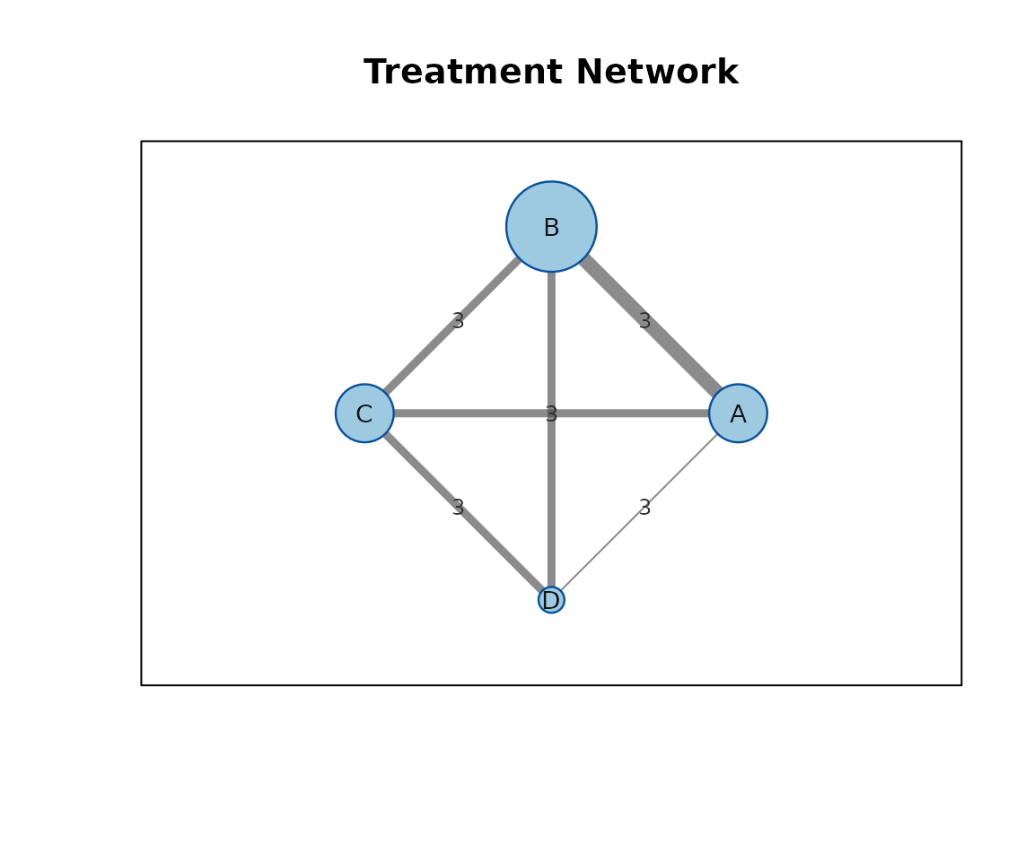
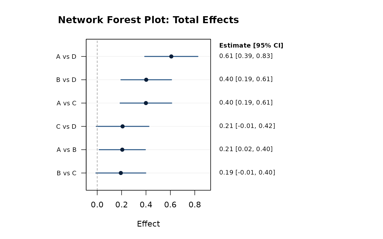
network_forest_plot() provides a standard forest plot
for one selected effect type ("direct",
"indirect", or "total").
network_forest_plot(
  nma_ml,
  effect_type = "total",
  order_by = "effect",
  right_digits = 2,
  main = "Network Forest Plot: Total Effects"
)
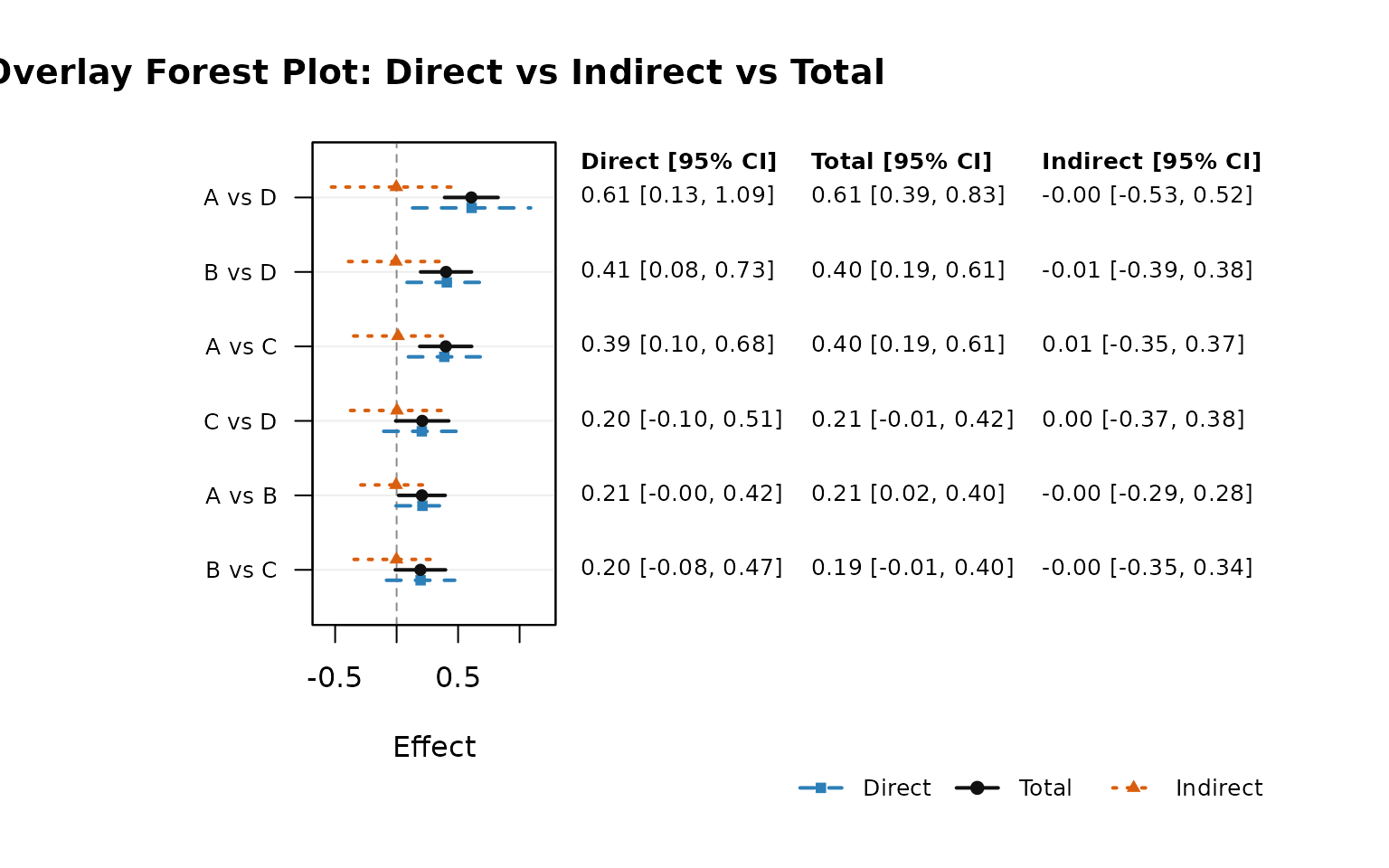
network_forest_overlay_plot() draws direct, total, and
indirect effects for each comparison using nearly overlapping lines for
fast visual comparison.
network_forest_overlay_plot(
  nma_ml,
  order_by = "total",
  right_label = "all",
  right_digits = 2,
  main = "Overlay Forest Plot: Direct vs Indirect vs Total"
)
Contribution Heatmap (Base R)
network_contribution_heatmap() visualizes the percentage
information contributed by each direct comparison estimate to each
network comparison.
network_contribution_heatmap(
  nma_ml,
  main = "Contribution Matrix Heatmap",
  show_values = FALSE
)
Arm-Level Pairwise Conversion
network_pairwise_data() converts arm-level binary or
continuous data to the contrast-level format used by
network_meta(). Binary examples can use log odds ratios
("OR"), log risk ratios ("RR"), or risk
differences ("RD"). Continuous examples can use mean
differences ("MD").
arm_dat <- data.frame(
  study = c("s1", "s1", "s1", "s2", "s2"),
  treatment = c("A", "B", "C", "A", "B"),
  event = c(4, 8, 10, 3, 6),
  n = c(40, 42, 41, 35, 37)
)

network_pairwise_data(
  arm_dat,
  study_id = "study",
  treatment = "treatment",
  event = "event",
  n = "n",
  effect_measure = "OR"
)
#>   study treatment_1 treatment_2    effect  variance effect_measure
#> 1    s1           A           B 0.7503056 0.4321895             OR
#> 2    s1           A           C 1.0658225 0.4100358             OR
#> 3    s1           B           C 0.3155169 0.2866698             OR
#> 4    s2           A           B 0.7248959 0.5635081             OR
Comparison-Adjusted Funnel Plot
Small-study diagnostics for network meta-analysis can center each observed contrast around the fitted network estimate for its comparison.
network_funnel_plot(nma_ml)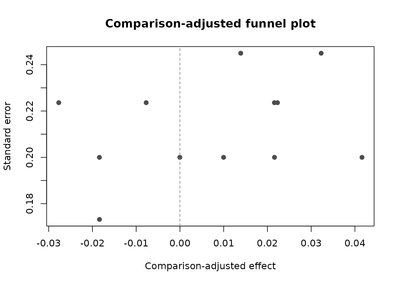
network_bias_test(nma_ml)$intercept
#>          term  estimate std_error  t_value   p_value
#> 1 (Intercept) 0.3492353 0.3109481 1.123131 0.2876223
Component Network Meta-analysis
When treatment names represent combinations of components,
network_component_meta() fits an additive component model
from a fitted nma_mars object. The example below treats
placebo as inactive and estimates the separate contributions of
components A and B.
component_dat <- data.frame(
  study = paste0("s", 1:8),
  trt1 = c("Placebo", "Placebo", "Placebo", "A", "B", "Placebo", "A", "B"),
  trt2 = c("A", "B", "A+B", "A+B", "A+B", "A+B", "A+B", "A+B"),
  yi = c(0.20, 0.30, 0.52, 0.31, 0.19, 0.48, 0.29, 0.21),
  vi = rep(0.04, 8)
)

component_nma <- network_meta(
  data = component_dat,
  study_id = "study",
  treatment_1 = "trt1",
  treatment_2 = "trt2",
  effect = "yi",
  variance = "vi",
  reference = "Placebo",
  model_type = "wls"
)

component_fit <- network_component_meta(component_nma, inactive = "Placebo")
component_fit$component_effects
#>   component estimate  std_error  ci_lower  ci_upper  z_value     p_value
#> A         A      0.2 0.09759001 0.0087271 0.3912729 2.049390 0.040423979
#> B         B      0.3 0.09759001 0.1087271 0.4912729 3.074085 0.002111491
component_fit$combinations
#>         treatment estimate  std_error  ci_lower  ci_upper observed_nma_effect
#> A               A      0.2 0.09759001 0.0087271 0.3912729                 0.2
#> A+B           A+B      0.5 0.10690450 0.2904710 0.7095290                 0.5
#> B               B      0.3 0.09759001 0.1087271 0.4912729                 0.3
#> Placebo   Placebo      0.0 0.00000000 0.0000000 0.0000000                 0.0
#>              residual
#> A        0.000000e+00
#> A+B     -1.110223e-16
#> B        0.000000e+00
#> Placebo  0.000000e+00
component_fit$fit_stats
#>     Q_additive df p_value rank singular
#> 1 1.848893e-30  1       1    2    FALSE
network_complex_effect() estimates arbitrary complex
interventions or comparisons from the component model.
network_complex_effect(component_fit, "A + B")
#>   intervention comparator estimate std_error ci_lower ci_upper
#> 1        A + B    Placebo      0.5 0.1069045 0.290471 0.709529
network_complex_effect(component_fit, intervention = "A+B", comparator = "A")
#>   intervention comparator estimate  std_error  ci_lower  ci_upper
#> 1          A+B          A      0.3 0.09759001 0.1087271 0.4912729
network_complex_effect(component_fit, 2)
#>   intervention comparator estimate std_error ci_lower ci_upper
#> 1        A + B    Placebo      0.5 0.1069045 0.290471 0.709529
Speed Controls
For larger networks, control can enable sparse matrix
algebra, reuse cached intermediate matrices, and parallelize selected
post-fit computations.
nma_ml_fast <- network_meta(
  data = nma_dat,
  study_id = "study",
  treatment_1 = "trt1",
  treatment_2 = "trt2",
  effect = "yi",
  variance = "vi",
  reference = "A",
  model_type = "multilevel",
  tau_components = "comparison",
  moderators = ~ severity + followup_months,
  estimation_method = "MLE",
  control = list(
    use_sparse = TRUE,
    reuse_inverses = TRUE,
    parallel = 2
  )
)

nma_ml_fast$control
Multivariate Network Meta-analysis
You can also fit in multivariate mode using
model_type = "multivariate". Use
within_varcov_type to choose the within-study covariance
structure used by the multivariate engine (for example
"multilevel"/"univariate" or metric-based
options such as "log_or" or
"smd_shared_control" when those required fields are
available). This example also includes moderators so one fitted object
shows the full cycle.
nma_mv <- suppressWarnings(network_meta(
  data = nma_dat,
  study_id = "study",
  treatment_1 = "trt1",
  treatment_2 = "trt2",
  effect = "yi",
  variance = "vi",
  reference = "A",
  model_type = "multivariate",
  heterogeneity = "flexible",
  moderators = c("severity", "followup_months"),
  estimation_method = "MLE",
  within_varcov_type = "multilevel"
))

summary(nma_mv)
#> Network Meta-analysis (MARS)
#> Model Type: multivariate
#> Heterogeneity: flexible
#> Moderators: severity, followup_months
#> Within-study covariance type: multilevel
#> Stored within-study covariance blocks: 11
#> Reference: A
#> Treatments: A, B, C, D
#>
#> Evidence Summary:
#> $n_comparisons_total
#> [1] 6
#>
#> $n_comparisons_with_direct
#> [1] 6
#>
#> $n_comparisons_with_indirect
#> [1] 6
#>
#> $n_comparisons_indirect_only
#> [1] 0
#>
#> $n_direct_effects
#> [1] 12
#>
#> $n_indirect_effects
#> [1] 48
#>
#>
#> Incoherence-Factor Assessment:
#> Global test:
#>  Q_incoherence df   p_value
#>       9.935036  6 0.1274146
#>
#> Per-comparison incoherence factors:
#>  treatment_1 treatment_2 incoherence_factor     if_se          z    p_value
#>            A           B          0.2682826 0.4318164  0.6212886 0.53440973
#>            A           C         -0.3675853 0.3107103 -1.1830483 0.23679000
#>            A           D         -0.5633495 0.3546375 -1.5885219 0.11216838
#>            B           C          0.1833119 0.4221076  0.4342776 0.66408688
#>            B           D         -0.3921117 0.2059983 -1.9034708 0.05697914
#>            C           D         -0.1668590 0.1238805 -1.3469346 0.17800131
#>    ci_lower   ci_upper
#>  -0.5780619 1.11462711
#>  -0.9765662 0.24139567
#>  -1.2584263 0.13172731
#>  -0.6440038 1.01062752
#>  -0.7958610 0.01163749
#>  -0.4096603 0.07594241
#>
#> Contribution Matrix (% information from direct comparisons):
#>        A vs B A vs C A vs D B vs C B vs D C vs D
#> A vs B      0   0.16   2.14      0  97.69   0.01
#> A vs C      0  99.87   0.11      0   0.00   0.02
#> A vs D      0   6.76  92.80      0   0.00   0.43
#> B vs C      0   4.89   1.81      0  93.29   0.02
#> B vs D      0   0.00   0.00      0 100.00   0.00
#> C vs D      0  72.80  26.93      0   0.00   0.27
#>
#> Model Fixed Effects (SE fallback applied when needed):
#>                            term    estimate std_error    z_value   p_value
#>  factor(data[[effectID]])A vs B  0.21372546 0.2217672  0.9637377 0.3351774
#>  factor(data[[effectID]])A vs C  0.36372546 0.3658167  0.9942833 0.3200849
#>  factor(data[[effectID]])A vs D  0.58372546 0.3724922  1.5670808 0.1170958
#>  factor(data[[effectID]])B vs C  0.20725491 0.2187216  0.9475742 0.3433463
#>  factor(data[[effectID]])B vs D  0.42973857 0.3122505  1.3762621 0.1687405
#>  factor(data[[effectID]])C vs D  0.20549028 0.1686609  1.2183633 0.2230860
#>                        severity  0.37254908 2.8438590  0.1310012 0.8957743
#>                 followup_months -0.02666667 0.1882336 -0.1416679 0.8873423
#>  se_source
#>    hessian
#>    hessian
#>    hessian
#>    hessian
#>    hessian
#>    hessian
#>    hessian
#>    hessian
#>
#> Fit Statistics:
#>  model_type heterogeneity n_treatments n_edges estimator       QE QE_df
#>        <NA>          <NA>            9       6       MLE 9.140389     6
#>       QE_p   logLik      Dev      AIC      BIC      AICc
#>  0.1658353 7.234778 9.530444 13.53044 20.31914 -126.4696
#>
#> Node-Splitting Assessment:
#>  Q_node_split df   p_value
#>      9.935036  6 0.1274146
#>
#>  treatment_1 treatment_2      direct     indirect direct_indirect_diff
#>            A           B 0.233333333 -0.034949264            0.2682826
#>            A           C 0.010410142  0.377995400           -0.3675853
#>            A           D 0.016375839  0.579725324           -0.5633495
#>            B           C 0.186666667  0.003354805            0.1833119
#>            B           D 0.002802677  0.394914417           -0.3921117
#>            C           D 0.020418327  0.187277295           -0.1668590
#>    diff_se          z    p_value   ci_lower   ci_upper
#>  0.4318164  0.6212886 0.53440973 -0.5780619 1.11462711
#>  0.3107103 -1.1830483 0.23679000 -0.9765662 0.24139567
#>  0.3546375 -1.5885219 0.11216838 -1.2584263 0.13172731
#>  0.4221076  0.4342776 0.66408688 -0.6440038 1.01062752
#>  0.2059983 -1.9034708 0.05697914 -0.7958610 0.01163749
#>  0.1238805 -1.3469346 0.17800131 -0.4096603 0.07594241
#>
#> Treatment Ranking:
#>  treatment mean_effect std_error mean_rank median_rank    sucra   sucr_a
#>          D   0.5961012 0.3545156     1.123           1 95.90000 95.90000
#>          C   0.3884055 0.3106587     2.170           2 61.00000 61.00000
#>          B   0.1983841 0.1938465     3.008           3 33.06667 33.06667
#>          A   0.0000000 0.0000000     3.699           4 10.03333 10.03333
#>   p_best
#>  0.90775
#>  0.03975
#>  0.00825
#>  0.04425
#>
#> Contribution Decomposition (top rows):
#> Fixed-Effect Design Diagnostics:
#> $rank
#> [1] 3
#>
#> $ncol
#> [1] 3
#>
#> $condition_number
#> [1] 43.11297
#>
#> $info_condition_number
#> [1] 1.999967
#>
#> $singular
#> [1] FALSE
#>
#> $near_singular
#> [1] FALSE
#>
#> $recommendation
#> [1] "No major fixed-effect rank/conditioning issues detected."
#>
#>
#> Treatment Order:
#>  rank treatment effect_vs_reference
#>     1         D              0.5961
#>     2         C              0.3884
#>     3         B              0.1984
#>     4         A              0.0000
#>
#> Direct / Indirect / Total Effects:
#>  treatment_1 treatment_2 direct direct_se direct_n_studies direct_n_effects
#>            A           B 0.2333    0.2728                3                3
#>            A           C 0.0104    0.0040                2                2
#>            A           D 0.0164    0.0066                1                1
#>            B           C 0.1867    0.2749                2                2
#>            B           D 0.0028    0.0011                2                2
#>            C           D 0.0204    0.0157                2                2
#>  direct_observed direct_observed_se indirect indirect_se indirect_n_paths
#>           0.2100             0.1095  -0.0349      0.3347                2
#>           0.3878             0.1491   0.3780      0.3107                2
#>           0.6100             0.2449   0.5797      0.3546                2
#>           0.1950             0.1414   0.0034      0.3203                2
#>           0.4082             0.1651   0.3949      0.2060                2
#>           0.2050             0.1581   0.1873      0.1229                2
#>  indirect_n_studies indirect_n_effects  total total_se total_n_studies
#>                   7                  7 0.1984   0.1938               9
#>                   8                  8 0.3884   0.3107               9
#>                   8                  9 0.5961   0.3545               9
#>                   8                  9 0.1900   0.1645              10
#>                   8                  8 0.3977   0.2060              10
#>                   7                  7 0.2077   0.1219               9
#>  total_n_effects direct_ci_lower direct_ci_upper direct_observed_ci_lower
#>               10         -0.3014          0.7681                  -0.0047
#>               10          0.0026          0.0183                   0.0956
#>               10          0.0035          0.0293                   0.1299
#>               11         -0.3521          0.7254                  -0.0822
#>               10          0.0006          0.0050                   0.0845
#>                9         -0.0104          0.0513                  -0.1049
#>  direct_observed_ci_upper indirect_ci_lower indirect_ci_upper total_ci_lower
#>                    0.4247           -0.6909            0.6210        -0.1815
#>                    0.6800           -0.2309            0.9869        -0.2205
#>                    1.0901           -0.1152            1.2747        -0.0987
#>                    0.4722           -0.6245            0.6312        -0.1324
#>                    0.7319           -0.0088            0.7987        -0.0060
#>                    0.5149           -0.0536            0.4281        -0.0311
#>  total_ci_upper
#>          0.5783
#>          0.9973
#>          1.2909
#>          0.5125
#>          0.8015
#>          0.4465
#>
#> Indirect SE note:
#> Indirect SEs are approximate; for mixed direct+indirect comparisons, var(indirect) is computed as var(total) + var(direct) assuming zero covariance.
#>
#> Heterogeneity Summary:
#> Overall Q:
#> $value
#>          [,1]
#> [1,] 9.140389
#>
#> $df
#> [1] 6
#>
#> $p
#>           [,1]
#> [1,] 0.1658353
#>
#>
#> Within-level Q:
#> $`A vs B`
#>  QE_value     QE_df      QE_p
#> 0.0400000 2.0000000 0.9801987
#>
#> $`A vs C`
#>  QE_value     QE_df      QE_p
#> 0.0160000 1.0000000 0.8993432
#>
#> $`A vs D`
#> [1] "only one effect size in this category"
#>
#> $`B vs C`
#>    QE_value       QE_df        QE_p
#> 0.001111111 1.000000000 0.973408772
#>
#> $`B vs D`
#>   QE_value      QE_df       QE_p
#> 0.01777778 1.00000000 0.89392977
#>
#> $`C vs D`
#>  QE_value     QE_df      QE_p
#> 0.0250000 1.0000000 0.8743671
#>
#>
#> Total I^2:
#> [1] 93.43997
#>
#> Within I^2:
#> [1]  0.002136528  0.002136528 95.528876009 95.528876009 95.528876009
#> [6] 95.528876009
#>
#> Between-study variance (tau^2):
#>  component  tau2
#>     A vs B 1e-06
#>     A vs C 1e-06
#>     A vs D 1e+00
#>     B vs C 1e+00
#>     B vs D 1e+00
#>     C vs D 1e+00
The moderator specification is stored in the fitted object:
nma_mv$moderators
#> [1] "severity"        "followup_months"
The output structure is the same, including effects, heterogeneity summaries, and treatment order:
nma_mv$effects
#>   treatment_1 treatment_2      direct   direct_se direct_n_studies
#> 1           A           B 0.233333333 0.272845092                3
#> 2           A           C 0.010410142 0.004001911                2
#> 3           A           D 0.016375839 0.006575811                1
#> 4           B           C 0.186666667 0.274873708                2
#> 5           B           D 0.002802677 0.001133923                2
#> 6           C           D 0.020418327 0.015748395                2
#>   direct_n_effects direct_observed direct_observed_se     indirect indirect_se
#> 1                3       0.2100000          0.1095445 -0.034949264   0.3346953
#> 2                2       0.3877778          0.1490712  0.377995400   0.3106845
#> 3                1       0.6100000          0.2449490  0.579725324   0.3545766
#> 4                2       0.1950000          0.1414214  0.003354805   0.3203424
#> 5                2       0.4081818          0.1651446  0.394914417   0.2059952
#> 6                2       0.2050000          0.1581139  0.187277295   0.1228754
#>   indirect_n_paths indirect_n_studies indirect_n_effects     total  total_se
#> 1                2                  7                  7 0.1983841 0.1938465
#> 2                2                  8                  8 0.3884055 0.3106587
#> 3                2                  8                  9 0.5961012 0.3545156
#> 4                2                  8                  9 0.1900215 0.1645105
#> 5                2                  8                  8 0.3977171 0.2059920
#> 6                2                  7                  7 0.2076956 0.1218621
#>   total_n_studies total_n_effects direct_ci_lower direct_ci_upper
#> 1               9              10   -0.3014332211     0.768099888
#> 2               9              10    0.0025665395     0.018253744
#> 3               9              10    0.0034874854     0.029264192
#> 4              10              11   -0.3520759020     0.725409235
#> 5              10              10    0.0005802281     0.005025125
#> 6               9               9   -0.0104479598     0.051284613
#>   direct_observed_ci_lower direct_observed_ci_upper indirect_ci_lower
#> 1             -0.004703297                0.4247033      -0.690939943
#> 2              0.095603598                0.6799520      -0.230935013
#> 3              0.129908832                1.0900912      -0.115231972
#> 4             -0.082180765                0.4721808      -0.624504774
#> 5              0.084504419                0.7318592      -0.008828698
#> 6             -0.104897516                0.5148975      -0.053554142
#>   indirect_ci_upper total_ci_lower total_ci_upper
#> 1         0.6210414   -0.181548166      0.5783163
#> 2         0.9869258   -0.220474353      0.9972854
#> 3         1.2746826   -0.098736612      1.2909389
#> 4         0.6312144   -0.132413166      0.5124561
#> 5         0.7986575   -0.006019905      0.8014541
#> 6         0.4281087   -0.031149628      0.4465409
nma_mv$evidence_summary
#> $n_comparisons_total
#> [1] 6
#>
#> $n_comparisons_with_direct
#> [1] 6
#>
#> $n_comparisons_with_indirect
#> [1] 6
#>
#> $n_comparisons_indirect_only
#> [1] 0
#>
#> $n_direct_effects
#> [1] 12
#>
#> $n_indirect_effects
#> [1] 48
nma_mv$indirect_se_note
#> [1] "Indirect SEs are approximate; for mixed direct+indirect comparisons, var(indirect) is computed as var(total) + var(direct) assuming zero covariance."
nma_mv$heterogeneity_summary
#> $Q_total
#> $Q_total$value
#>          [,1]
#> [1,] 9.140389
#>
#> $Q_total$df
#> [1] 6
#>
#> $Q_total$p
#>           [,1]
#> [1,] 0.1658353
#>
#>
#> $Q_within
#> $Q_within$`A vs B`
#>  QE_value     QE_df      QE_p
#> 0.0400000 2.0000000 0.9801987
#>
#> $Q_within$`A vs C`
#>  QE_value     QE_df      QE_p
#> 0.0160000 1.0000000 0.8993432
#>
#> $Q_within$`A vs D`
#> [1] "only one effect size in this category"
#>
#> $Q_within$`B vs C`
#>    QE_value       QE_df        QE_p
#> 0.001111111 1.000000000 0.973408772
#>
#> $Q_within$`B vs D`
#>   QE_value      QE_df       QE_p
#> 0.01777778 1.00000000 0.89392977
#>
#> $Q_within$`C vs D`
#>  QE_value     QE_df      QE_p
#> 0.0250000 1.0000000 0.8743671
#>
#>
#> $Q_by_level
#> NULL
#>
#> $I2_total
#> [1] 93.43997
#>
#> $I2_within
#> [1]  0.002136528  0.002136528 95.528876009 95.528876009 95.528876009
#> [6] 95.528876009
#>
#> $level_heterogeneity
#> NULL
#>
#> $tau2
#>   component  tau2
#> 1    A vs B 1e-06
#> 2    A vs C 1e-06
#> 3    A vs D 1e+00
#> 4    B vs C 1e+00
#> 5    B vs D 1e+00
#> 6    C vs D 1e+00
nma_mv$heterogeneity_summary$tau2
#>   component  tau2
#> 1    A vs B 1e-06
#> 2    A vs C 1e-06
#> 3    A vs D 1e+00
#> 4    B vs C 1e+00
#> 5    B vs D 1e+00
#> 6    C vs D 1e+00
nma_mv$incoherence_assessment$global
#>   Q_incoherence df   p_value
#> 1      9.935036  6 0.1274146
nma_mv$incoherence_assessment$per_comparison
#>   treatment_1 treatment_2 incoherence_factor     if_se          z    p_value
#> 1           A           B          0.2682826 0.4318164  0.6212886 0.53440973
#> 2           A           C         -0.3675853 0.3107103 -1.1830483 0.23679000
#> 3           A           D         -0.5633495 0.3546375 -1.5885219 0.11216838
#> 4           B           C          0.1833119 0.4221076  0.4342776 0.66408688
#> 5           B           D         -0.3921117 0.2059983 -1.9034708 0.05697914
#> 6           C           D         -0.1668590 0.1238805 -1.3469346 0.17800131
#>     ci_lower   ci_upper
#> 1 -0.5780619 1.11462711
#> 2 -0.9765662 0.24139567
#> 3 -1.2584263 0.13172731
#> 4 -0.6440038 1.01062752
#> 5 -0.7958610 0.01163749
#> 6 -0.4096603 0.07594241
nma_mv$contribution_matrix
#>              A vs B       A vs C       A vs D       B vs C       B vs D
#> A vs B 4.499323e-10 1.563275e-01 2.144864e+00 3.812357e-10 9.768878e+01
#> A vs C 2.202187e-11 9.986814e+01 1.123532e-01 6.890900e-10 2.739690e-05
#> A vs D 1.818523e-08 6.762164e+00 9.280012e+01 1.534226e-08 3.903011e-03
#> B vs C 3.807219e-10 4.885075e+00 1.807110e+00 6.710233e-10 9.328982e+01
#> B vs D 5.142455e-13 1.023784e-09 2.423296e-09 4.917517e-13 1.000000e+02
#> C vs D 5.277409e-09 7.279891e+01 2.693127e+01 9.482879e-09 1.688052e-03
#>              C vs D
#> A vs B 1.002643e-02
#> A vs C 1.948361e-02
#> A vs D 4.338121e-01
#> B vs C 1.799203e-02
#> B vs D 1.688253e-11
#> C vs D 2.681312e-01
nma_mv$treatment_order
#>   rank treatment effect_vs_reference
#> 1    1         D           0.5961012
#> 2    2         C           0.3884055
#> 3    3         B           0.1983841
#> 4    4         A           0.0000000
nma_mv$node_splitting$global
#>   Q_node_split df   p_value
#> 1     9.935036  6 0.1274146
nma_mv$ranking$rankings
#>   treatment mean_effect std_error mean_rank median_rank    sucra   sucr_a
#> D         D   0.5961012 0.3545156     1.123           1 95.90000 95.90000
#> C         C   0.3884055 0.3106587     2.170           2 61.00000 61.00000
#> B         B   0.1983841 0.1938465     3.008           3 33.06667 33.06667
#> A         A   0.0000000 0.0000000     3.699           4 10.03333 10.03333
#>    p_best
#> D 0.90775
#> C 0.03975
#> B 0.00825
#> A 0.04425
nma_mv$fit_stats
#>   model_type heterogeneity n_treatments n_edges estimator       QE QE_df
#> 1       <NA>          <NA>            9       6       MLE 9.140389     6
#>        QE_p   logLik      Dev      AIC      BIC      AICc
#> 1 0.1658353 7.234778 9.530444 13.53044 20.31914 -126.4696
nma_mv$level_heterogeneity_summary
#> NULL
nma_mv$heterogeneity_summary$level_heterogeneity
#> NULL
Multivariate Variants
For multivariate NMA where studies contribute multiple outcomes or
multiple contrasts, cluster-robust SEs can be requested by setting
robustID:
nma_mv_cluster <- suppressWarnings(network_meta(
  data = nma_dat,
  study_id = "study",
  treatment_1 = "trt1",
  treatment_2 = "trt2",
  effect = "yi",
  variance = "vi",
  reference = "A",
  model_type = "multivariate",
  heterogeneity = "flexible",
  moderators = c("severity", "followup_months"),
  estimation_method = "MLE",
  within_varcov_type = "multilevel",
  robustID = "study"
))

nma_mv_cluster$fit_coefficients
nma_mv_cluster$robust_cluster_id
network_forest_plot(nma_mv, effect_type = "total", main = "Multivariate: Total")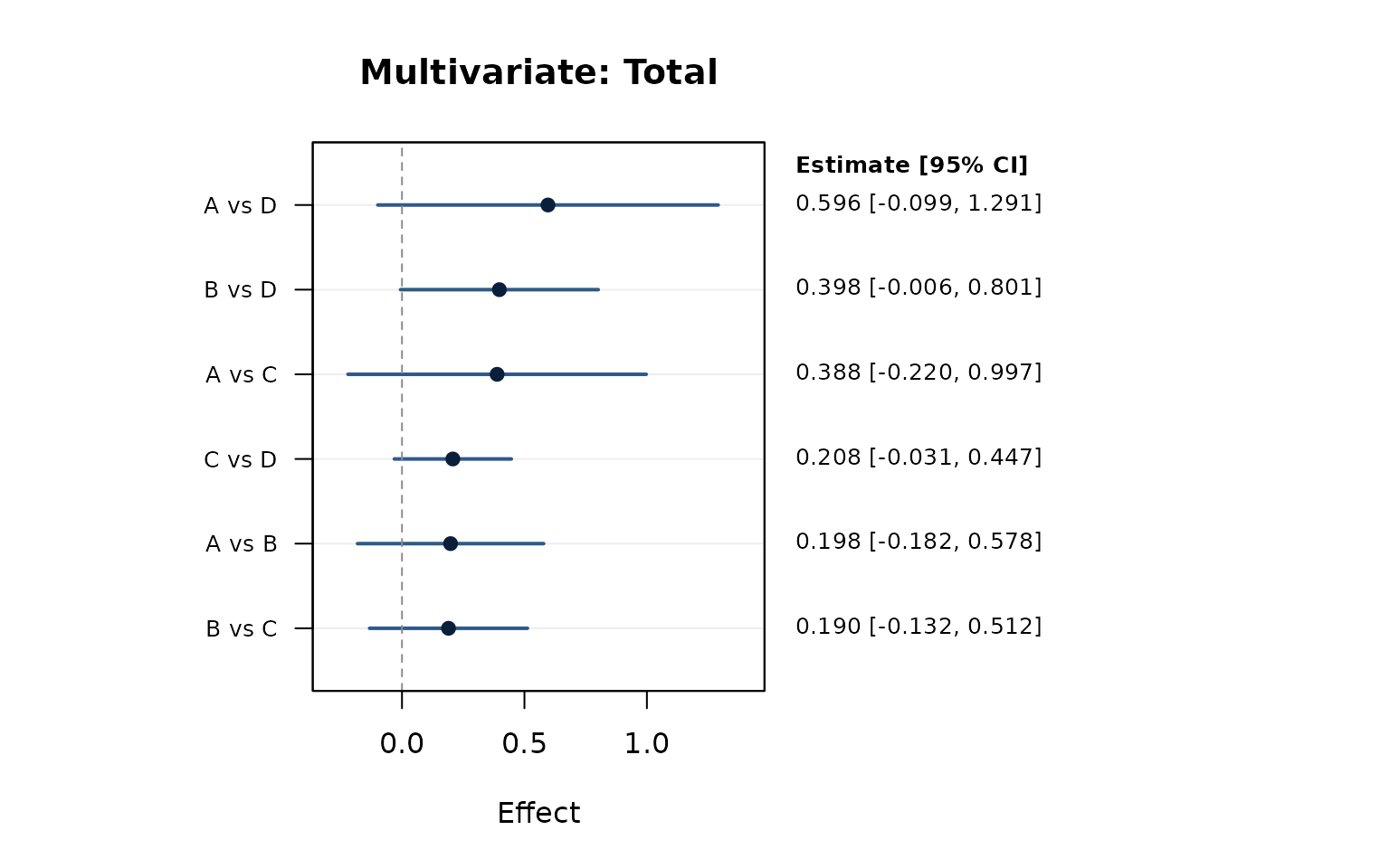
network_forest_overlay_plot(nma_mv, order_by = "total", right_label = "total",
                            main = "Multivariate: Overlay")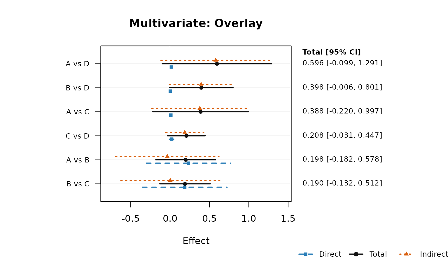
network_contribution_heatmap(nma_mv, main = "Multivariate: Contribution")
Compare multilevel and multivariate model fit side-by-side on the same dataset
mars:::compare_nma_models(
  multilevel = nma_ml,
  multivariate = nma_mv
)
#>                model_type heterogeneity n_treatments n_edges estimator       QE
#> multilevel     multilevel      flexible            4       6       MLE 0.106132
#> multivariate multivariate      flexible            4       6       MLE 9.140389
#>              QE_df      QE_p   logLik       Dev       AIC      BIC      AICc
#> multilevel       7 0.9999972 3.609517 16.780967  6.780967 10.17531 -133.2190
#> multivariate     6 0.1658353 7.234778  9.530444 13.530444 20.31914 -126.4696
#>              AIC_rank BIC_rank AICc_rank
#> multilevel          1        1         1
#> multivariate        2        2         2