Alternative Estimation Frameworks with `mars`

This vignette demonstrates three alternative estimation frameworks available in mars:

Bootstrap
Jackknife (leave-one-cluster-out for multilevel models)
Permutation

For each framework, we show how to obtain:

Point estimate from the empirical distribution of replicate estimates
95% interval (2.5%, 97.5%) from that same distribution

library(mars)

extract_alt_interval <- function(x, term = "(Intercept)") {
  if (!is.null(x$summary) &&
      all(c("point_estimate", "ci_lower", "ci_upper") %in% colnames(x$summary)) &&
      term %in% rownames(x$summary)) {
    out <- x$summary[term, c("point_estimate", "ci_lower", "ci_upper"), drop = FALSE]
    return(out)
  }

  if (!is.null(x$summary) &&
      all(c("estimate", "ci_lower", "ci_upper") %in% colnames(x$summary)) &&
      term %in% rownames(x$summary)) {
    out <- x$summary[term, c("estimate", "ci_lower", "ci_upper"), drop = FALSE]
    names(out) <- c("point_estimate", "ci_lower", "ci_upper")
    return(out)
  }

  if (!is.null(x$quantiles) &&
      all(c("2.5%", "50.0%", "97.5%") %in% colnames(x$quantiles)) &&
      term %in% rownames(x$quantiles)) {
    out <- x$quantiles[term, c("50.0%", "2.5%", "97.5%"), drop = FALSE]
    names(out) <- c("point_estimate", "ci_lower", "ci_upper")
    return(out)
  }

  if (!is.null(x$summary) &&
      all(c("estimate", "jackknife_se") %in% colnames(x$summary)) &&
      term %in% rownames(x$summary)) {
    est <- x$summary[term, "estimate"]
    se <- x$summary[term, "jackknife_se"]
    out <- data.frame(
      point_estimate = est,
      ci_lower = est - 1.96 * se,
      ci_upper = est + 1.96 * se,
      row.names = term
    )
    return(out)
  }

  stop("Could not extract a point estimate + interval for term: ", term)
}

Data and Base Model

We use the bundled school dataset and a multilevel model.

fit <- mars(
  formula = effect ~ 1 + (1 | district/study),
  data = school,
  studyID = "district",
  variance = "var",
  varcov_type = "multilevel",
  structure = "multilevel",
  estimation_method = "MLE"
)

summary(fit)
#> Results generated with MARS:v 0.5.1.1 
#> Thursday, April  2, 2026
#> 
#> Model Type: 
#> multilevel
#> 
#> Estimation Method: 
#> Maximum Likelihood
#> 
#> Model Formula: 
#> effect ~ 1 + (1 | district/study)
#> 
#> Data Summary: 
#> Number of Effect Sizes: 56
#> Number of Fixed Effects: 1
#> Number of Random Effects: 2
#> 
#> Random Data Summary: 
#> Number unique district: 11 
#> Number unique study: 56
#> 
#> Random Components: 
#>      term     var     SD
#>  district 0.05774 0.2403
#>     study 0.03286 0.1813
#> 
#> Fixed Effects Estimates: 
#>    attribute estimate      SE z_test p_value   lower  upper
#>  (Intercept)   0.1845 0.08048  2.292 0.02191 0.02671 0.3422
#> 
#> Model Fit Statistics: 
#>  logLik   Dev   AIC   BIC AICc
#>  -8.395 24.79 22.79 28.87 24.5
#> 
#> Q Error: 578.864 (55), p < 0.0001
#> 
#> I2 (General): 
#>     names values
#>  district  92.38
#>     study  87.34
#> 
#> I2 (Jackson): 98.69621
#> I2 (Between): 86.3727
#> 
#> Residual Diagnostics: 
#>   n n_finite_raw mean_raw sd_raw   rmse    mae q_pearson mean_abs_studentized
#>  56           56 -0.06446 0.3258 0.3293 0.2632      96.8                1.065
#>  max_abs_studentized prop_abs_studentized_gt2 prop_abs_studentized_gt3
#>                4.196                   0.1071                  0.03571
#> 
#> Normality (whitened residuals):                   test n_tested statistic p_value
#>  shapiro_wilk_whitened       56    0.9555 0.03766
#> 
#> Heteroscedasticity trend (|raw residual| ~ fitted):   n corr_abs_raw_fitted slope p_value
#>  56                  NA    NA      NA

Bootstrap

set.seed(2026)
boot_repl <- replicate_bootstrap(
  number_bootstraps = 10,
  data = school,
  formula = effect ~ 1 + (1 | district/study),
  studyID = "district",
  effectID = NULL,
  sample_size = NULL,
  variance = "var",
  varcov_type = "multilevel",
  structure = "multilevel",
  estimation_method = "MLE"
)

boot_stats <- compute_alt_stats(boot_repl, type = "bootstrap")

The summary component contains distribution-based point estimates and 95% intervals:

summary(boot_stats)
#> Results generated with MARS:v 0.5.1.1 
#> Thursday, April 02, 2026 
#> 
#> Model Type:
#> multilevel 
#> 
#> Estimation Method:
#> MLE 
#> 
#> Robust Method:
#> Bootstrap
#> Number of Replications: 10 
#> 
#> Model Formula:
#> effect ~ 1 + (1 | district/study) 
#> 
#> Data Summary:
#> Number of Effect Sizes: 56 
#> Number of Fixed Effects: 1 
#> Number of Random Effects: 2 
#> 
#> Random Components (Bootstrap CIs):
#> Variances:
#>          50%   2.5%  97.5%
#> Tau_1 0.0633 0.0120 0.0941
#> Tau_2 0.0208 0.0081 0.0257
#> 
#> SDs:
#>             50%   2.5%  97.5%
#> district 0.2513 0.1094 0.3066
#> study    0.1442 0.0897 0.1604
#> 
#> Fixed Effects Estimates (Bootstrap CIs):
#>                50%   2.5%  97.5%
#> (Intercept) 0.1269 0.0121 0.1968
#> 
#> Model Fit Statistics (Bootstrap CIs):
#>             50%     2.5%    97.5%
#> logLik -10.8166 -46.9168   6.5048
#> Dev     29.6333  -5.0095 101.8335
#> AIC     27.6333  -7.0095  99.8335
#> BIC     33.7359  -0.9295 105.7935
#> AICc    29.3304  -5.2967 101.6268

The quantiles component provides named quantile columns directly:

boot_stats$quantiles["(Intercept)", c("2.5%", "50.0%", "97.5%")]
#>       2.5%      50.0%      97.5% 
#> 0.01207444 0.12689320 0.19679377

All coefficient distributions can also be visualized in a single base R figure, with one histogram panel per effect:

plot(boot_stats)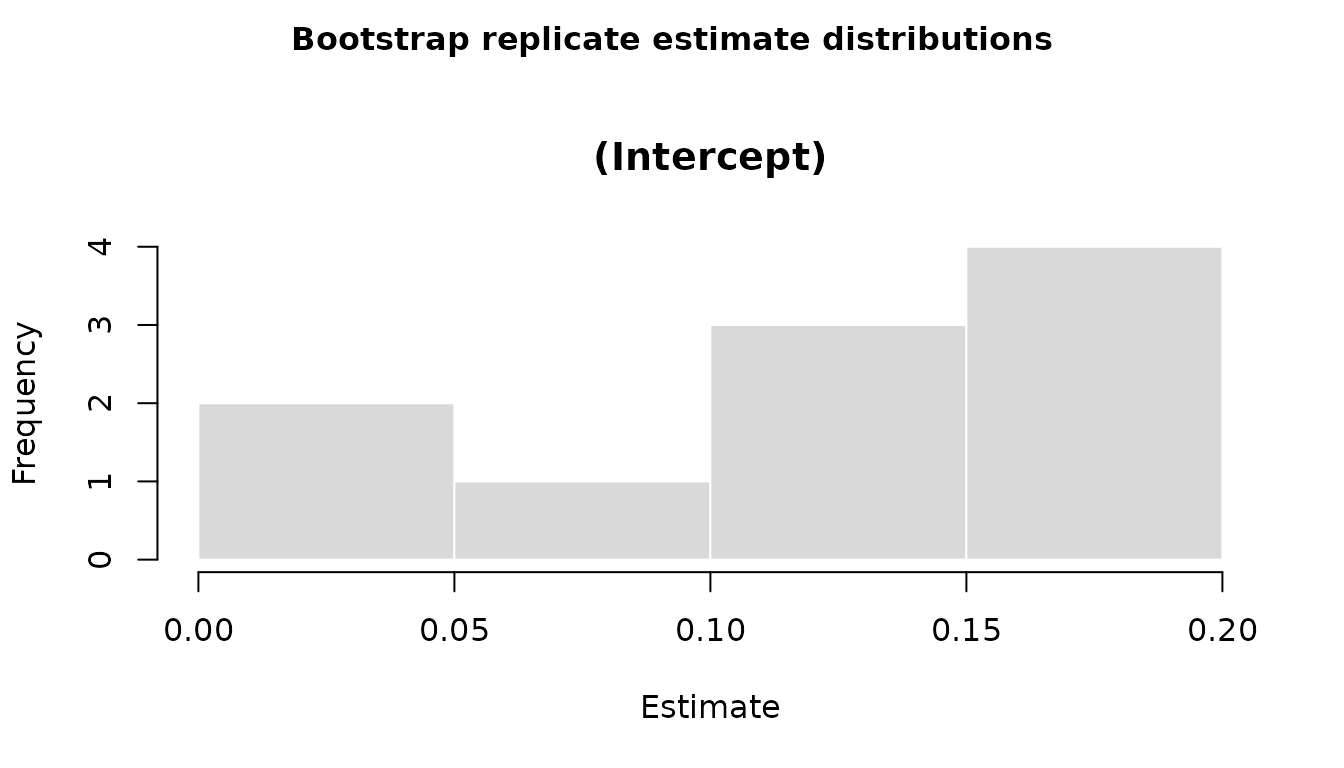

Jackknife

For multilevel models, jackknife leaves out one highest-level cluster at a time (here: one district per replication).

set.seed(2026)
jack_repl <- replicate_jackknife(
  data = school,
  structure = "multilevel",
  formula = effect ~ 1 + (1 | district/study),
  studyID = "district",
  effectID = NULL,
  sample_size = NULL,
  variance = "var",
  varcov_type = "multilevel",
  estimation_method = "MLE"
)

jack_stats <- compute_alt_stats(jack_repl, type = "jackknife")

Jackknife summaries include both the distribution-based interval and a classic jackknife standard error:

summary(jack_stats)
#> Results generated with MARS:v 0.5.1.1 
#> Thursday, April 02, 2026 
#> 
#> Model Type:
#> multilevel 
#> 
#> Estimation Method:
#> MLE 
#> 
#> Robust Method:
#> Jackknife
#> Number of Replications: 11 
#> 
#> Model Formula:
#> effect ~ 1 + (1 | district/study) 
#> 
#> Data Summary:
#> Number of Effect Sizes: 52 
#> Number of Fixed Effects: 1 
#> Number of Random Effects: 2 
#> 
#> Random Components (Jackknife CIs):
#> Variances:
#>          50%   2.5%  97.5%
#> Tau_1 0.0604 0.0307 0.0670
#> Tau_2 0.0332 0.0220 0.0467
#> 
#> SDs:
#>             50%   2.5%  97.5%
#> district 0.2457 0.1722 0.2589
#> study    0.1821 0.1481 0.2161
#> 
#> Fixed Effects Estimates (Jackknife CIs):
#>                50%   2.5%  97.5%
#> (Intercept) 0.1953 0.1297 0.2102
#> 
#> Model Fit Statistics (Jackknife CIs):
#>            50%     2.5%   97.5%
#> logLik -7.7962 -11.8631 -0.2970
#> Dev    23.5924   8.5940 31.7263
#> AIC    21.5924   6.5940 29.7263
#> BIC    27.4461  12.4760 35.2915
#> AICc   23.4590   8.4408 31.8155

Permutation

For multilevel models, permutation shuffles highest-level clusters while keeping rows within each cluster together.

set.seed(2026)
perm_repl <- mars_alt_estimation(
  type = "permutation",
  number_permutations = 10,
  data = school,
  structure = "multilevel",
  formula = effect ~ 1 + (1 | district/study),
  studyID = "district",
  effectID = NULL,
  sample_size = NULL,
  variance = "var",
  varcov_type = "multilevel",
  estimation_method = "MLE"
)

perm_stats <- compute_alt_stats(perm_repl, type = "permutation")

Permutation uses the same summary structure as bootstrap:

summary(perm_stats)
#> Results generated with MARS:v 0.5.1.1 
#> Thursday, April 02, 2026 
#> 
#> Model Type:
#> multilevel 
#> 
#> Estimation Method:
#> MLE 
#> 
#> Robust Method:
#> Permutation
#> Number of Replications: 10 
#> 
#> Model Formula:
#> effect ~ 1 + (1 | district/study) 
#> 
#> Data Summary:
#> Number of Effect Sizes: 56 
#> Number of Fixed Effects: 1 
#> Number of Random Effects: 2 
#> 
#> Random Components (Permutation CIs):
#> Variances:
#>          50%   2.5%  97.5%
#> Tau_1 0.0577 0.0577 0.0577
#> Tau_2 0.0329 0.0329 0.0329
#> 
#> SDs:
#>             50%   2.5%  97.5%
#> district 0.2403 0.2403 0.2403
#> study    0.1813 0.1813 0.1813
#> 
#> Fixed Effects Estimates (Permutation CIs):
#>                50%   2.5%  97.5%
#> (Intercept) 0.1255 0.1038 0.1646
#> 
#> Model Fit Statistics (Permutation CIs):
#>            50%    2.5%   97.5%
#> logLik -8.3949 -8.3949 -8.3949
#> Dev    24.7899 24.7899 24.7899
#> AIC    22.7899 22.7899 22.7899
#> BIC    28.8659 28.8659 28.8659
#> AICc   24.5042 24.5042 24.5042

Compare the Three Frameworks

The example below extracts the intercept summaries side-by-side.

comparison <- rbind(
  bootstrap = extract_alt_interval(boot_stats),
  jackknife = extract_alt_interval(jack_stats),
  permutation = extract_alt_interval(perm_stats)
)

comparison
#>             point_estimate   ci_lower  ci_upper
#> bootstrap        0.1268932 0.01207444 0.1967938
#> jackknife        0.1952655 0.12967311 0.2101858
#> permutation      0.1255471 0.10375708 0.1646467

In practice, increase the number of replications for stable inference (for example, 500 to 2000+), especially for interval estimation.

`mars` authors

2026-04-02

Data and Base Model

Bootstrap

Jackknife

Permutation

Compare the Three Frameworks

Alternative Estimation Frameworks with mars

mars authors

2026-04-02

Data and Base Model

Bootstrap

Jackknife

Permutation

Compare the Three Frameworks

Alternative Estimation Frameworks with `mars`

`mars` authors