Publication Bias Models with MARS
mars authors
2026-05-15
Publication-Bias-Models.RmdThis vignette demonstrates publication-bias modeling with
publication_bias(method = "beta_selection") and
publication_bias(method = "beta_binomial") and
publication_bias(method = "logistic_selection") after
fitting mars models.
Current implementation note: - Univariate publication-bias fits
estimate a scalar tau2 inside the selection model. -
Multilevel and multivariate publication-bias fits use the fitted MARS
covariance blocks directly, rather than collapsing to diagonal sampling
variances. - Reported standard errors use a conservative rule: when both
Hessian-based and OPG-based SEs are finite, the larger value is
reported.
library(mars)
extract_full_data_coefficients <- function(fit) {
  est_raw <- if(!is.null(fit$beta_r)) {
    fit$beta_r
  } else if(!is.null(fit$beta_fe)) {
    fit$beta_fe
  } else {
    fit$est_values$mu
  }

  est_vec <- as.numeric(est_raw)
  est_names <- names(est_raw)
  if(is.matrix(est_raw) || is.data.frame(est_raw)) {
    est_vec <- as.numeric(est_raw[, 1, drop = TRUE])
    est_names <- rownames(est_raw)
  }
  if(length(est_names) != length(est_vec)) {
    est_names <- colnames(fit$design_matrix)
  }

  se_vec <- rep(NA_real_, length(est_vec))
  vc <- fit$varcov_beta
  if(is.matrix(vc) && nrow(vc) == length(est_vec)) {
    se_vec <- sqrt(pmax(diag(vc), 0))
    if(!is.null(colnames(vc)) && length(colnames(vc)) == length(est_vec)) {
      est_names <- colnames(vc)
    }
  }

  data.frame(
    term = est_names,
    estimate = est_vec,
    std_error = se_vec,
    stringsAsFactors = FALSE
  )
}

compare_pub_bias_3 <- function(x, y, z,
                               label_x = "beta_selection",
                               label_y = "beta_binomial",
                               label_z = "logistic_selection",
                               ref = NULL,
                               label_ref = "all_data") {
  a <- x$coefficients
  b <- y$coefficients
  c <- z$coefficients
  names(a)[names(a) == "estimate"] <- paste0("estimate_", label_x)
  names(a)[names(a) == "std_error"] <- paste0("se_", label_x)
  names(b)[names(b) == "estimate"] <- paste0("estimate_", label_y)
  names(b)[names(b) == "std_error"] <- paste0("se_", label_y)
  names(c)[names(c) == "estimate"] <- paste0("estimate_", label_z)
  names(c)[names(c) == "std_error"] <- paste0("se_", label_z)

  out <- merge(
    a[, c("term", paste0("estimate_", label_x), paste0("se_", label_x))],
    b[, c("term", paste0("estimate_", label_y), paste0("se_", label_y))],
    by = "term",
    all = TRUE
  )
  out <- merge(
    out,
    c[, c("term", paste0("estimate_", label_z), paste0("se_", label_z))],
    by = "term",
    all = TRUE
  )
  if(!is.null(ref)) {
    r <- ref
    names(r)[names(r) == "estimate"] <- paste0("estimate_", label_ref)
    names(r)[names(r) == "std_error"] <- paste0("se_", label_ref)
    out <- merge(
      out,
      r[, c("term", paste0("estimate_", label_ref), paste0("se_", label_ref))],
      by = "term",
      all = TRUE
    )
  }
  out[order(out$term), ]
}

plot_pub_bias_compare_3 <- function(tbl,
                                    label_x = "beta_selection",
                                    label_y = "beta_binomial",
                                    label_z = "logistic_selection",
                                    label_ref = "all_data",
                                    main = "Method Comparison") {
  ref_est_name <- paste0("estimate_", label_ref)
  ref_se_name <- paste0("se_", label_ref)
  est_x <- tbl[[paste0("estimate_", label_x)]]
  se_x <- tbl[[paste0("se_", label_x)]]
  est_y <- tbl[[paste0("estimate_", label_y)]]
  se_y <- tbl[[paste0("se_", label_y)]]
  est_z <- tbl[[paste0("estimate_", label_z)]]
  se_z <- tbl[[paste0("se_", label_z)]]
  has_ref <- ref_est_name %in% names(tbl)
  est_ref <- if(has_ref) tbl[[ref_est_name]] else rep(NA_real_, nrow(tbl))
  se_ref <- if(has_ref && ref_se_name %in% names(tbl)) tbl[[ref_se_name]] else rep(NA_real_, nrow(tbl))
  k <- nrow(tbl)
  xpos <- seq_len(k)
  offsets <- if(has_ref) c(-0.27, -0.09, 0.09, 0.27) else c(-0.18, 0, 0.18)
  all_vals <- c(
    est_x, est_y, est_z, est_ref,
    est_x - 1.96 * se_x, est_x + 1.96 * se_x,
    est_y - 1.96 * se_y, est_y + 1.96 * se_y,
    est_z - 1.96 * se_z, est_z + 1.96 * se_z,
    est_ref - 1.96 * se_ref, est_ref + 1.96 * se_ref
  )
  ylim <- range(all_vals[is.finite(all_vals)])
  old_par <- par(no.readonly = TRUE)
  on.exit(par(old_par), add = TRUE)
  x_axis_cex <- max(0.55, min(0.8, 8 / max(nchar(tbl$term), 1L)))
  mar <- old_par$mar
  mar[1] <- max(mar[1], 8 + 3 * x_axis_cex)
  par(mar = mar)

  plot(xpos, est_x, type = "n", xaxt = "n", xlab = "", ylab = "Estimate", main = main, ylim = ylim)
  abline(h = 0, lty = 2, col = "gray60")
  axis(1, at = xpos, labels = tbl$term, las = 2, cex.axis = x_axis_cex)
  title(xlab = "Coefficient Term", line = 6)

  keep_x <- is.finite(est_x) & is.finite(se_x)
  keep_y <- is.finite(est_y) & is.finite(se_y)
  keep_z <- is.finite(est_z) & is.finite(se_z)
  keep_ref <- has_ref & is.finite(est_ref) & is.finite(se_ref)
  pt_x <- is.finite(est_x)
  pt_y <- is.finite(est_y)
  pt_z <- is.finite(est_z)
  pt_ref <- has_ref & is.finite(est_ref)
  miss_se_x <- is.finite(est_x) & !is.finite(se_x)
  miss_se_y <- is.finite(est_y) & !is.finite(se_y)
  miss_se_z <- is.finite(est_z) & !is.finite(se_z)
  miss_se_ref <- has_ref & is.finite(est_ref) & !is.finite(se_ref)
  x_x <- xpos + offsets[1]
  x_y <- xpos + offsets[2]
  x_z <- xpos + offsets[3]
  x_ref <- if(has_ref) xpos + offsets[4] else xpos
  if(any(keep_x)) {
    segments(x_x[keep_x], est_x[keep_x] - 1.96 * se_x[keep_x],
             x_x[keep_x], est_x[keep_x] + 1.96 * se_x[keep_x], col = "#1F78B4", lwd = 2)
  }
  if(any(keep_y)) {
    segments(x_y[keep_y], est_y[keep_y] - 1.96 * se_y[keep_y],
             x_y[keep_y], est_y[keep_y] + 1.96 * se_y[keep_y], col = "#E31A1C", lwd = 2)
  }
  if(any(keep_z)) {
    segments(x_z[keep_z], est_z[keep_z] - 1.96 * se_z[keep_z],
             x_z[keep_z], est_z[keep_z] + 1.96 * se_z[keep_z], col = "#33A02C", lwd = 2)
  }
  if(any(keep_ref)) {
    segments(x_ref[keep_ref], est_ref[keep_ref] - 1.96 * se_ref[keep_ref],
             x_ref[keep_ref], est_ref[keep_ref] + 1.96 * se_ref[keep_ref], col = "#4D4D4D", lwd = 2)
  }
  if(any(pt_x)) {
    points(x_x[pt_x], est_x[pt_x], pch = 19, col = "#1F78B4")
  }
  if(any(pt_y)) {
    points(x_y[pt_y], est_y[pt_y], pch = 17, col = "#E31A1C")
  }
  if(any(pt_z)) {
    points(x_z[pt_z], est_z[pt_z], pch = 15, col = "#33A02C")
  }
  if(any(pt_ref)) {
    points(x_ref[pt_ref], est_ref[pt_ref], pch = 18, col = "#4D4D4D")
  }
  if(any(miss_se_x)) {
    points(x_x[miss_se_x], est_x[miss_se_x], pch = 1, col = "#1F78B4", cex = 1.2, lwd = 1.5)
  }
  if(any(miss_se_y)) {
    points(x_y[miss_se_y], est_y[miss_se_y], pch = 2, col = "#E31A1C", cex = 1.2, lwd = 1.5)
  }
  if(any(miss_se_z)) {
    points(x_z[miss_se_z], est_z[miss_se_z], pch = 0, col = "#33A02C", cex = 1.2, lwd = 1.5)
  }
  if(any(miss_se_ref)) {
    points(x_ref[miss_se_ref], est_ref[miss_se_ref], pch = 5, col = "#4D4D4D", cex = 1.2, lwd = 1.5)
  }

  legend_labels <- c(label_x, label_y, label_z)
  legend_cols <- c("#1F78B4", "#E31A1C", "#33A02C")
  legend_pch <- c(19, 17, 15)
  if(has_ref) {
    legend_labels <- c(legend_labels, label_ref)
    legend_cols <- c(legend_cols, "#4D4D4D")
    legend_pch <- c(legend_pch, 18)
  }
  legend("topright", legend = legend_labels, col = legend_cols, pch = legend_pch, bty = "n")
  if(any(miss_se_x) || any(miss_se_y) || any(miss_se_z) || any(miss_se_ref)) {
    mtext("Open symbols indicate estimates with unavailable SE.", side = 3, line = 0.2, cex = 0.8)
  }
}

extract_alt_interval <- function(x, term = "(Intercept)") {
  if(!is.null(x$summary) &&
     all(c("point_estimate", "ci_lower", "ci_upper") %in% colnames(x$summary)) &&
     term %in% rownames(x$summary)) {
    out <- x$summary[term, c("point_estimate", "ci_lower", "ci_upper"), drop = FALSE]
    return(out)
  }

  if(!is.null(x$summary) &&
     all(c("estimate", "ci_lower", "ci_upper") %in% colnames(x$summary)) &&
     term %in% rownames(x$summary)) {
    out <- x$summary[term, c("estimate", "ci_lower", "ci_upper"), drop = FALSE]
    names(out) <- c("point_estimate", "ci_lower", "ci_upper")
    return(out)
  }

  stop("Could not extract a point estimate + interval for term: ", term)
}
Univariate Example
fit_uni <- mars(
  formula = yi ~ 1,
  data = bcg,
  studyID = "trial",
  variance = "vi",
  varcov_type = "univariate",
  structure = "univariate",
  estimation_method = "MLE"
)

summary(fit_uni)
#> Results generated with MARS:v 0.5.2
#> Friday, May 15, 2026
#>
#> Model Type:
#> univariate
#>
#> Estimation Method:
#> Maximum Likelihood
#>
#> Model Formula:
#> yi ~ 1
#>
#> Data Summary:
#> Number of Effect Sizes: 13
#> Number of Fixed Effects: 1
#> Number of Random Effects: 1
#>
#> Random Components:
#>       term  var     SD
#>  intercept 0.28 0.5292
#>
#> Fixed Effects Estimates:
#>    attribute estimate     SE z_test   p_value  lower   upper
#>  (Intercept)  -0.7112 0.1719 -4.137 3.513e-05 -1.048 -0.3743
#>
#> Model Fit Statistics:
#>  logLik   Dev   AIC   BIC AICc
#>  -12.67 31.33 29.33 30.46 37.9
#>
#> Q Error: 152.233 (12), p < 0.0001
#>
#> I2 (General): 92.03957
#>
#> Residual Diagnostics:
#>   n n_finite_raw mean_raw sd_raw   rmse    mae q_pearson mean_abs_studentized
#>  13           13 -0.02945 0.6938 0.6672 0.5958     13.16               0.9527
#>  max_abs_studentized prop_abs_studentized_gt2 prop_abs_studentized_gt3
#>                1.434                        0                        0
#>
#> Normality (whitened residuals):                   test n_tested statistic p_value
#>  shapiro_wilk_whitened       13     0.886 0.08592
#>
#> Heteroscedasticity trend (|raw residual| ~ fitted):   n corr_abs_raw_fitted slope p_value
#>  13                  NA    NA      NA
pb_uni <- publication_bias(
  fit_uni,
  method = "beta_selection",
  p_value_tail = "two.sided",
  maxit = 100,
  integration_points = 31
)

summary(pb_uni)
#> Publication Bias Model (MARS)
#> Method: beta_selection
#> Structure: univariate
#> Effects: 13  | Studies: 13
#> P-value tail: two.sided
#> Convergence: 0 - Converged
#> Objective: 9.147
#>
#> Selection Parameters:
#>  parameter estimate
#>      alpha   1.1797
#>       beta   0.0008
#>       tau2   0.4513
#>
#> Selection Weight Profile (p-value grid):
#>           model p_value  weight
#>  beta_selection  0.0100  0.4415
#>  beta_selection  0.1189  0.7740
#>  beta_selection  0.2278  0.9924
#>  beta_selection  0.3367  1.2392
#>  beta_selection  0.4456  1.5590
#>  beta_selection  0.5544  2.0173
#>  beta_selection  0.6633  2.7566
#>  beta_selection  0.7722  4.1858
#>  beta_selection  0.8811  8.2075
#>  beta_selection  0.9900 99.4385
#>
#> Bias-Adjusted Coefficients:
#>         term estimate std_error z_value p_value
#>  (Intercept)  -1.3572     0.252 -5.3848       0
#>
#> Adjusted vs Unadjusted Summary:
#>         term unadjusted_estimate unadjusted_se unadjusted_ci_lower
#>  (Intercept)             -0.7112        0.1719             -1.0481
#>  unadjusted_ci_upper estimate std_error adjusted_ci_lower adjusted_ci_upper
#>              -0.3743  -1.3572     0.252           -1.8512           -0.8632
#>  estimate_diff percent_change direction_changed ci_overlap
#>         -0.646       -90.8364             FALSE       TRUE
#>
#> Small-Study Effects Check (Egger-type):
#> Model: SND ~ precision
#> Method: Egger-type small-study-effects regression with study-cluster robust SE (CR1)
#> Intercept: -7.8519 SE: 3.2091 t: -2.4468 df: 12 p: 0.0308
#>
#> SE note:
#> SE rule: reported SEs use the larger of the Hessian-based and OPG-based values when both are finite, otherwise the finite one.
pb_uni_bb <- publication_bias(
  fit_uni,
  method = "beta_binomial",
  n_bins = 8,
  p_value_tail = "two.sided",
  maxit = 100,
  integration_points = 31
)

summary(pb_uni_bb)
#> Publication Bias Model (MARS)
#> Method: beta_binomial
#> Structure: univariate
#> Effects: 13  | Studies: 13
#> P-value tail: two.sided
#> Convergence: 0 - Converged
#> Objective: -33.37
#>
#> Selection Parameters:
#>  parameter  estimate
#>      alpha 7213.1265
#>       beta    0.0006
#>       tau2    1.6265
#>     n_bins    8.0000
#>
#> Selection Weight Profile (bin probabilities):
#>  bin p_lower p_upper weight
#>    1   0.000   0.125      0
#>    2   0.125   0.250      0
#>    3   0.250   0.375      0
#>    4   0.375   0.500      0
#>    5   0.500   0.625      0
#>    6   0.625   0.750      0
#>    7   0.750   0.875      0
#>    8   0.875   1.000      1
#>
#> Bias-Adjusted Coefficients:
#>         term estimate std_error z_value p_value
#>  (Intercept)   0.3576    0.4306  0.8304  0.4063
#>
#> Adjusted vs Unadjusted Summary:
#>         term unadjusted_estimate unadjusted_se unadjusted_ci_lower
#>  (Intercept)             -0.7112        0.1719             -1.0481
#>  unadjusted_ci_upper estimate std_error adjusted_ci_lower adjusted_ci_upper
#>              -0.3743   0.3576    0.4306           -0.4864            1.2016
#>  estimate_diff percent_change direction_changed ci_overlap
#>         1.0688       150.2788              TRUE       TRUE
#>
#> Small-Study Effects Check (Egger-type):
#> Model: SND ~ precision
#> Method: Egger-type small-study-effects regression with study-cluster robust SE (CR1)
#> Intercept: -7.8519 SE: 3.2091 t: -2.4468 df: 12 p: 0.0308
#>
#> SE note:
#> SE rule: reported SEs use the larger of the Hessian-based and OPG-based values when both are finite, otherwise the finite one. beta_binomial uses discretized p-value bins; coefficient magnitudes can differ materially from beta_selection.
pb_uni_logit <- publication_bias(
  fit_uni,
  method = "logistic_selection",
  p_value_tail = "two.sided",
  maxit = 100,
  integration_points = 31
)

summary(pb_uni_logit)
#> Publication Bias Model (MARS)
#> Method: logistic_selection
#> Structure: univariate
#> Effects: 13  | Studies: 13
#> P-value tail: two.sided
#> Convergence: 0 - Converged
#> Objective: 13.92
#>
#> Selection Parameters:
#>        parameter estimate
#>  logit_intercept   8.0045
#>      logit_slope   0.5688
#>             tau2   0.4256
#>
#> Selection Weight Profile (p-value grid):
#>               model p_value weight
#>  logistic_selection  0.0100 1.0000
#>  logistic_selection  0.1189 0.9999
#>  logistic_selection  0.2278 0.9999
#>  logistic_selection  0.3367 0.9998
#>  logistic_selection  0.4456 0.9998
#>  logistic_selection  0.5544 0.9998
#>  logistic_selection  0.6633 0.9997
#>  logistic_selection  0.7722 0.9997
#>  logistic_selection  0.8811 0.9997
#>  logistic_selection  0.9900 0.9997
#>
#> Bias-Adjusted Coefficients:
#>         term estimate std_error z_value p_value
#>  (Intercept)  -0.7723    0.2848 -2.7119  0.0067
#>
#> Adjusted vs Unadjusted Summary:
#>         term unadjusted_estimate unadjusted_se unadjusted_ci_lower
#>  (Intercept)             -0.7112        0.1719             -1.0481
#>  unadjusted_ci_upper estimate std_error adjusted_ci_lower adjusted_ci_upper
#>              -0.3743  -0.7723    0.2848           -1.3305           -0.2141
#>  estimate_diff percent_change direction_changed ci_overlap
#>        -0.0611        -8.5908             FALSE       TRUE
#>
#> Small-Study Effects Check (Egger-type):
#> Model: SND ~ precision
#> Method: Egger-type small-study-effects regression with study-cluster robust SE (CR1)
#> Intercept: -7.8519 SE: 3.2091 t: -2.4468 df: 12 p: 0.0308
#>
#> SE note:
#> SE rule: reported SEs use the larger of the Hessian-based and OPG-based values when both are finite, otherwise the finite one.
Selection and adjusted fixed effects:
pb_uni$selection
#>        alpha         beta         tau2
#> 1.1797078025 0.0008305913 0.4512552801
pb_uni$covariance_mode
#> [1] "publication_bias_tau2"
pb_uni$coefficients
#>          term  estimate std_error   z_value      p_value
#> 1 (Intercept) -1.357227   0.25205 -5.384754 7.254387e-08
pb_uni_bb$selection_weights
#>   bin p_lower p_upper       weight
#> 1   1   0.000   0.125 4.187106e-28
#> 2   2   0.125   0.250 3.523234e-24
#> 3   3   0.250   0.375 1.524843e-20
#> 4   4   0.375   0.500 4.583461e-17
#> 5   5   0.500   0.625 1.102277e-13
#> 6   6   0.625   0.750 2.385876e-10
#> 7   7   0.750   0.875 5.737124e-07
#> 8   8   0.875   1.000 9.999994e-01
pb_uni_logit$selection
#> logit_intercept     logit_slope            tau2
#>       8.0045371       0.5687618       0.4255908
pb_uni_logit$coefficients
#>          term   estimate std_error   z_value     p_value
#> 1 (Intercept) -0.7722971 0.2847817 -2.711892 0.006690042
For the univariate case, the publication-bias likelihood still
estimates a scalar tau2, so the selection parameter vector
includes tau2 along with the selection-function
parameters.
ref_uni <- extract_full_data_coefficients(fit_uni)
cmp_uni <- compare_pub_bias_3(pb_uni, pb_uni_bb, pb_uni_logit, ref = ref_uni)
cmp_uni
#>          term estimate_beta_selection se_beta_selection estimate_beta_binomial
#> 1 (Intercept)               -1.357227           0.25205              0.3575826
#>   se_beta_binomial estimate_logistic_selection se_logistic_selection
#> 1        0.4306209                  -0.7722971             0.2847817
#>   estimate_all_data se_all_data
#> 1        -0.7111991   0.1718968
plot_pub_bias_compare_3(cmp_uni, main = "Univariate: publication-bias methods with all-data reference")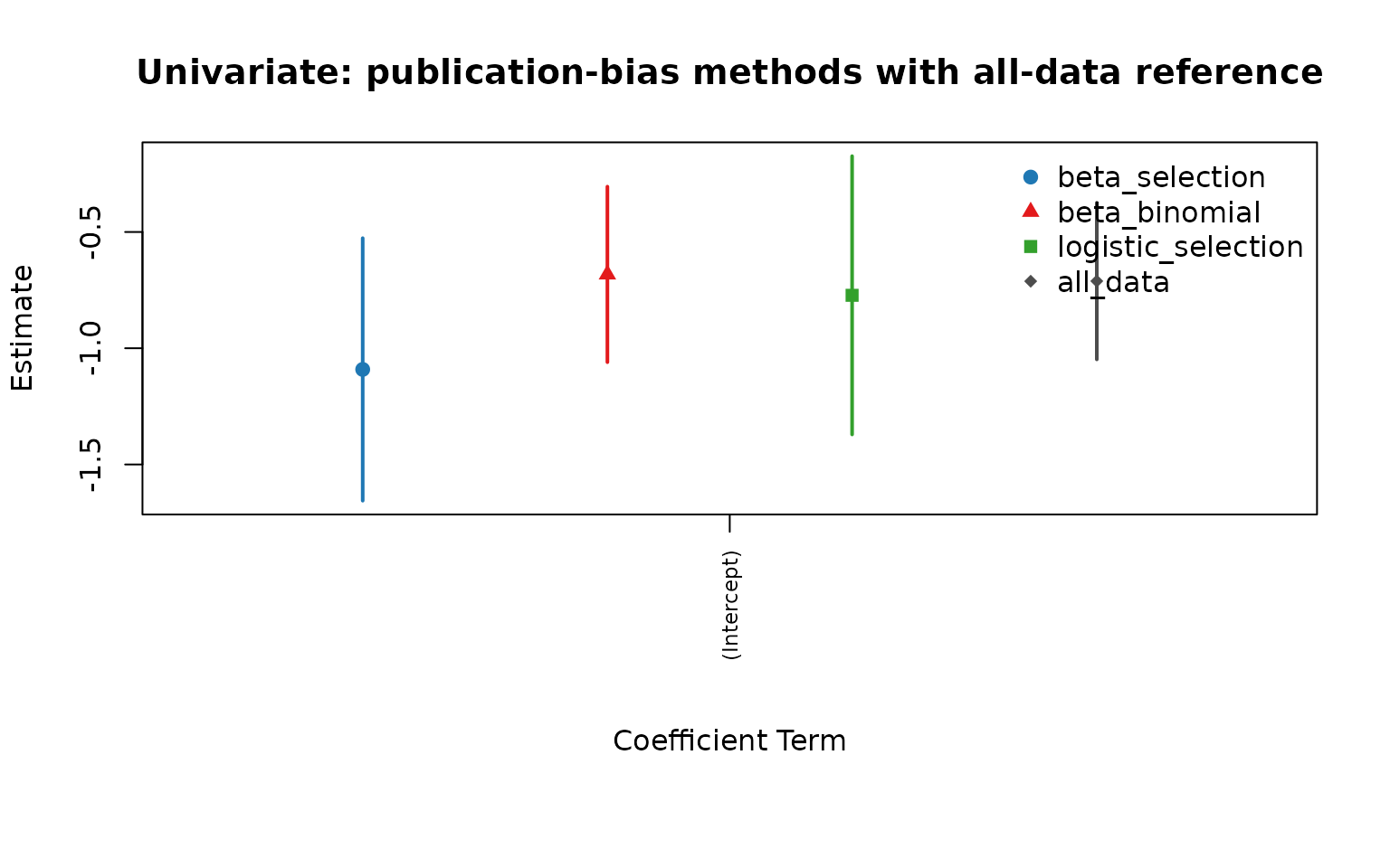
Funnel plot from the publication-bias fit:
funnel_plot(pb_uni)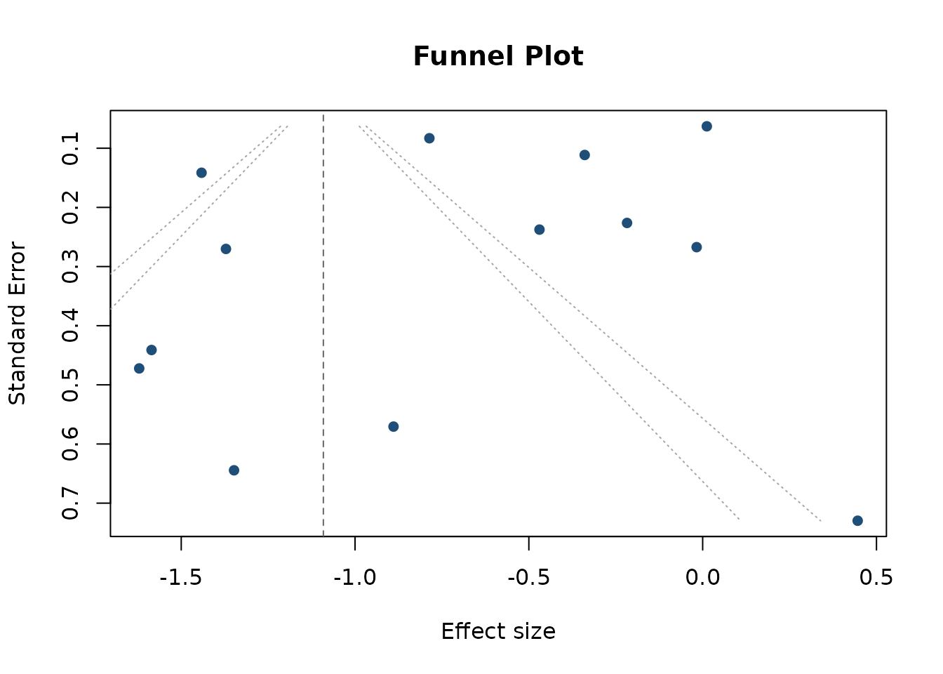
Jackknife version of the complete-data fit and each publication-bias model:
set.seed(2026)

# Keep the vignette jackknife examples intentionally small/lightweight.
bcg_jack <- bcg[seq_len(min(6, nrow(bcg))), , drop = FALSE]

jack_complete <- mars_alt_estimation(
  type = "jackknife",
  data = bcg_jack,
  formula = yi ~ 1,
  studyID = "trial",
  effectID = NULL,
  sample_size = NULL,
  variance = "vi",
  varcov_type = "univariate",
  structure = "univariate",
  estimation_method = "MLE",
  jackknife_target = "complete_data"
)

jack_beta_selection <- mars_alt_estimation(
  type = "jackknife",
  data = bcg_jack,
  formula = yi ~ 1,
  studyID = "trial",
  effectID = NULL,
  sample_size = NULL,
  variance = "vi",
  varcov_type = "univariate",
  structure = "univariate",
  estimation_method = "MLE",
  jackknife_target = "beta_selection",
  publication_bias_args = list(
    p_value_tail = "two.sided",
    maxit = 100,
    integration_points = 31
  )
)

jack_beta_binomial <- mars_alt_estimation(
  type = "jackknife",
  data = bcg_jack,
  formula = yi ~ 1,
  studyID = "trial",
  effectID = NULL,
  sample_size = NULL,
  variance = "vi",
  varcov_type = "univariate",
  structure = "univariate",
  estimation_method = "MLE",
  jackknife_target = "beta_binomial",
  publication_bias_args = list(
    p_value_tail = "two.sided",
    n_bins = 8,
    maxit = 100,
    integration_points = 31
  )
)

jack_logistic <- mars_alt_estimation(
  type = "jackknife",
  data = bcg_jack,
  formula = yi ~ 1,
  studyID = "trial",
  effectID = NULL,
  sample_size = NULL,
  variance = "vi",
  varcov_type = "univariate",
  structure = "univariate",
  estimation_method = "MLE",
  jackknife_target = "logistic_selection",
  publication_bias_args = list(
    p_value_tail = "two.sided",
    maxit = 100,
    integration_points = 31
  )
)

jack_complete_stats <- compute_alt_stats(jack_complete, type = "jackknife")
jack_beta_selection_stats <- compute_alt_stats(jack_beta_selection, type = "jackknife")
jack_beta_binomial_stats <- compute_alt_stats(jack_beta_binomial, type = "jackknife")
jack_logistic_stats <- compute_alt_stats(jack_logistic, type = "jackknife")

jackknife_compare <- rbind(
  complete_data = extract_alt_interval(jack_complete_stats),
  beta_selection = extract_alt_interval(jack_beta_selection_stats),
  beta_binomial = extract_alt_interval(jack_beta_binomial_stats),
  logistic_selection = extract_alt_interval(jack_logistic_stats)
)

jackknife_compare
The univariate jackknife illustration uses only the first six trials so the vignette demonstrates the workflow without refitting all leave-one-out models from the full dataset.
jack_est <- jackknife_compare[, "point_estimate"]
jack_lo <- jackknife_compare[, "ci_lower"]
jack_hi <- jackknife_compare[, "ci_upper"]
xpos <- seq_len(nrow(jackknife_compare))

plot(
  xpos, jack_est,
  ylim = range(c(jack_lo, jack_hi)),
  xaxt = "n", xlab = "", ylab = "Jackknife Estimate",
  pch = 19, col = "#1F78B4",
  main = "Univariate Jackknife: complete data and publication-bias targets"
)
segments(xpos, jack_lo, xpos, jack_hi, lwd = 2, col = "#1F78B4")
abline(h = 0, lty = 2, col = "gray60")
axis(1, at = xpos, labels = rownames(jackknife_compare), las = 2)
title(xlab = "Jackknife Target", line = 6)
Multilevel Example
fit_ml <- mars(
  formula = effect ~ 1 + (1 | district/study),
  data = school,
  studyID = "district",
  variance = "var",
  varcov_type = "multilevel",
  structure = "multilevel",
  estimation_method = "MLE"
)

summary(fit_ml)
#> Results generated with MARS:v 0.5.2
#> Friday, May 15, 2026
#>
#> Model Type:
#> multilevel
#>
#> Estimation Method:
#> Maximum Likelihood
#>
#> Model Formula:
#> effect ~ 1 + (1 | district/study)
#>
#> Data Summary:
#> Number of Effect Sizes: 56
#> Number of Fixed Effects: 1
#> Number of Random Effects: 2
#>
#> Random Data Summary:
#> Number unique district: 11
#> Number unique study: 56
#>
#> Random Components:
#>      term     var     SD
#>  district 0.05774 0.2403
#>     study 0.03286 0.1813
#>
#> Fixed Effects Estimates:
#>    attribute estimate      SE z_test p_value   lower  upper
#>  (Intercept)   0.1845 0.08048  2.292 0.02191 0.02671 0.3422
#>
#> Model Fit Statistics:
#>  logLik   Dev   AIC   BIC AICc
#>  -8.395 24.79 22.79 28.87 24.5
#>
#> Q Error: 578.864 (55), p < 0.0001
#>
#> I2 (General):
#>     names values
#>  district  92.38
#>     study  87.34
#>
#> I2 (Jackson): 98.69621
#> I2 (Between): 86.3727
#>
#> Residual Diagnostics:
#>   n n_finite_raw mean_raw sd_raw   rmse    mae q_pearson mean_abs_studentized
#>  56           56 -0.06446 0.3258 0.3293 0.2632      96.8                1.065
#>  max_abs_studentized prop_abs_studentized_gt2 prop_abs_studentized_gt3
#>                4.196                   0.1071                  0.03571
#>
#> Normality (whitened residuals):                   test n_tested statistic p_value
#>  shapiro_wilk_whitened       56    0.9555 0.03766
#>
#> Heteroscedasticity trend (|raw residual| ~ fitted):   n corr_abs_raw_fitted slope p_value
#>  56                  NA    NA      NA
pb_ml <- publication_bias(
  fit_ml,
  method = "beta_selection",
  p_value_tail = "two.sided",
  maxit = 100,
  integration_points = 31
)

summary(pb_ml)
#> Publication Bias Model (MARS)
#> Method: beta_selection
#> Structure: multilevel
#> Effects: 56  | Studies: 11
#> P-value tail: two.sided
#> Convergence: 0 - Converged
#> Objective: -142.5
#>
#> Selection Parameters:
#>  parameter  estimate
#>      alpha 2179.5386
#>       beta    0.0003
#>
#> Selection Weight Profile (p-value grid):
#>           model p_value weight
#>  beta_selection  0.0100      0
#>  beta_selection  0.1189      0
#>  beta_selection  0.2278      0
#>  beta_selection  0.3367      0
#>  beta_selection  0.4456      0
#>  beta_selection  0.5544      0
#>  beta_selection  0.6633      0
#>  beta_selection  0.7722      0
#>  beta_selection  0.8811      0
#>  beta_selection  0.9900      0
#>
#> Bias-Adjusted Coefficients:
#>         term estimate std_error z_value p_value
#>  (Intercept)   0.9456    0.0332 28.4619       0
#>
#> Adjusted vs Unadjusted Summary:
#>         term unadjusted_estimate unadjusted_se unadjusted_ci_lower
#>  (Intercept)              0.1845        0.0805              0.0267
#>  unadjusted_ci_upper estimate std_error adjusted_ci_lower adjusted_ci_upper
#>               0.3422   0.9456    0.0332            0.8805            1.0107
#>  estimate_diff percent_change direction_changed ci_overlap
#>         0.7611       412.6349             FALSE      FALSE
#>
#> Small-Study Effects Check (Egger-type):
#> Model: SND ~ precision
#> Method: Egger-type small-study-effects regression with study-cluster robust SE (CR1)
#> Intercept: 3.69 SE: 1.8503 t: 1.9943 df: 10 p: 0.0741
#>
#> SE note:
#> SE rule: reported SEs use the larger of the Hessian-based and OPG-based values when both are finite, otherwise the finite one. Covariance structure: used the fitted MARS within/between-study covariance blocks directly for the publication-bias likelihood.
pb_ml_bb <- publication_bias(
  fit_ml,
  method = "beta_binomial",
  n_bins = 8,
  p_value_tail = "two.sided",
  maxit = 100,
  integration_points = 31
)

summary(pb_ml_bb)
#> Publication Bias Model (MARS)
#> Method: beta_binomial
#> Structure: multilevel
#> Effects: 56  | Studies: 11
#> P-value tail: two.sided
#> Convergence: 0 - Converged
#> Objective: -400.3
#>
#> Selection Parameters:
#>  parameter estimate
#>      alpha 158.6092
#>       beta   0.8091
#>     n_bins   8.0000
#>
#> Selection Weight Profile (bin probabilities):
#>  bin p_lower p_upper weight
#>    1   0.000   0.125 0.0000
#>    2   0.125   0.250 0.0000
#>    3   0.250   0.375 0.0000
#>    4   0.375   0.500 0.0000
#>    5   0.500   0.625 0.0000
#>    6   0.625   0.750 0.0011
#>    7   0.750   0.875 0.0332
#>    8   0.875   1.000 0.9656
#>
#> Bias-Adjusted Coefficients:
#>         term estimate std_error z_value p_value
#>  (Intercept)   1.2761     0.034 37.5353       0
#>
#> Adjusted vs Unadjusted Summary:
#>         term unadjusted_estimate unadjusted_se unadjusted_ci_lower
#>  (Intercept)              0.1845        0.0805              0.0267
#>  unadjusted_ci_upper estimate std_error adjusted_ci_lower adjusted_ci_upper
#>               0.3422   1.2761     0.034            1.2094            1.3427
#>  estimate_diff percent_change direction_changed ci_overlap
#>         1.0916       591.7976             FALSE      FALSE
#>
#> Small-Study Effects Check (Egger-type):
#> Model: SND ~ precision
#> Method: Egger-type small-study-effects regression with study-cluster robust SE (CR1)
#> Intercept: 3.69 SE: 1.8503 t: 1.9943 df: 10 p: 0.0741
#>
#> SE note:
#> SE rule: reported SEs use the larger of the Hessian-based and OPG-based values when both are finite, otherwise the finite one. Covariance structure: used the fitted MARS within/between-study covariance blocks directly for the publication-bias likelihood. beta_binomial uses discretized p-value bins; coefficient magnitudes can differ materially from beta_selection.
pb_ml_logit <- publication_bias(
  fit_ml,
  method = "logistic_selection",
  p_value_tail = "two.sided",
  maxit = 100,
  integration_points = 31
)

summary(pb_ml_logit)
#> Publication Bias Model (MARS)
#> Method: logistic_selection
#> Structure: multilevel
#> Effects: 56  | Studies: 11
#> P-value tail: two.sided
#> Convergence: 0 - Converged
#> Objective: 8.396
#>
#> Selection Parameters:
#>        parameter estimate
#>  logit_intercept   7.8501
#>      logit_slope  11.7805
#>
#> Selection Weight Profile (p-value grid):
#>               model p_value weight
#>  logistic_selection  0.0100 1.0000
#>  logistic_selection  0.1189 1.0000
#>  logistic_selection  0.2278 1.0000
#>  logistic_selection  0.3367 1.0000
#>  logistic_selection  0.4456 1.0000
#>  logistic_selection  0.5544 1.0000
#>  logistic_selection  0.6633 1.0000
#>  logistic_selection  0.7722 1.0000
#>  logistic_selection  0.8811 0.9999
#>  logistic_selection  0.9900 0.9997
#>
#> Bias-Adjusted Coefficients:
#>         term estimate std_error z_value p_value
#>  (Intercept)   0.1844     0.087  2.1183  0.0341
#>
#> Adjusted vs Unadjusted Summary:
#>         term unadjusted_estimate unadjusted_se unadjusted_ci_lower
#>  (Intercept)              0.1845        0.0805              0.0267
#>  unadjusted_ci_upper estimate std_error adjusted_ci_lower adjusted_ci_upper
#>               0.3422   0.1844     0.087            0.0138             0.355
#>  estimate_diff percent_change direction_changed ci_overlap
#>         -1e-04        -0.0299             FALSE       TRUE
#>
#> Small-Study Effects Check (Egger-type):
#> Model: SND ~ precision
#> Method: Egger-type small-study-effects regression with study-cluster robust SE (CR1)
#> Intercept: 3.69 SE: 1.8503 t: 1.9943 df: 10 p: 0.0741
#>
#> SE note:
#> SE rule: reported SEs use the larger of the Hessian-based and OPG-based values when both are finite, otherwise the finite one. Covariance structure: used the fitted MARS within/between-study covariance blocks directly for the publication-bias likelihood.
Multilevel coefficients with standard errors:
pb_ml$covariance_mode
#> [1] "fixed_mars_structure"
pb_ml$covariance_structure
#> $structure
#> [1] "multilevel"
#>
#> $Tau
#>            [,1]       [,2]
#> [1,] 0.05773805 0.00000000
#> [2,] 0.00000000 0.03286473
pb_ml$coefficients
#>          term  estimate  std_error  z_value       p_value
#> 1 (Intercept) 0.9455827 0.03322272 28.46192 3.469368e-178
pb_ml_bb$coefficients
#>          term estimate std_error  z_value       p_value
#> 1 (Intercept) 1.276058 0.0339962 37.53531 2.446214e-308
pb_ml_logit$coefficients
#>          term  estimate  std_error  z_value    p_value
#> 1 (Intercept) 0.1844002 0.08704963 2.118334 0.03414679
For multilevel fits, publication_bias() now uses the
fitted MARS block covariance structure directly. In that case the output
stores covariance_mode = "fixed_mars_structure" and the
publication-bias selection parameters no longer include a separate
scalar tau2.
ref_ml <- extract_full_data_coefficients(fit_ml)
cmp_ml <- compare_pub_bias_3(pb_ml, pb_ml_bb, pb_ml_logit, ref = ref_ml)
cmp_ml
#>          term estimate_beta_selection se_beta_selection estimate_beta_binomial
#> 1 (Intercept)               0.9455827        0.03322272               1.276058
#>   se_beta_binomial estimate_logistic_selection se_logistic_selection
#> 1        0.0339962                   0.1844002            0.08704963
#>   estimate_all_data se_all_data
#> 1         0.1844554   0.0804815
plot_pub_bias_compare_3(cmp_ml, main = "Multilevel: publication-bias methods with all-data reference")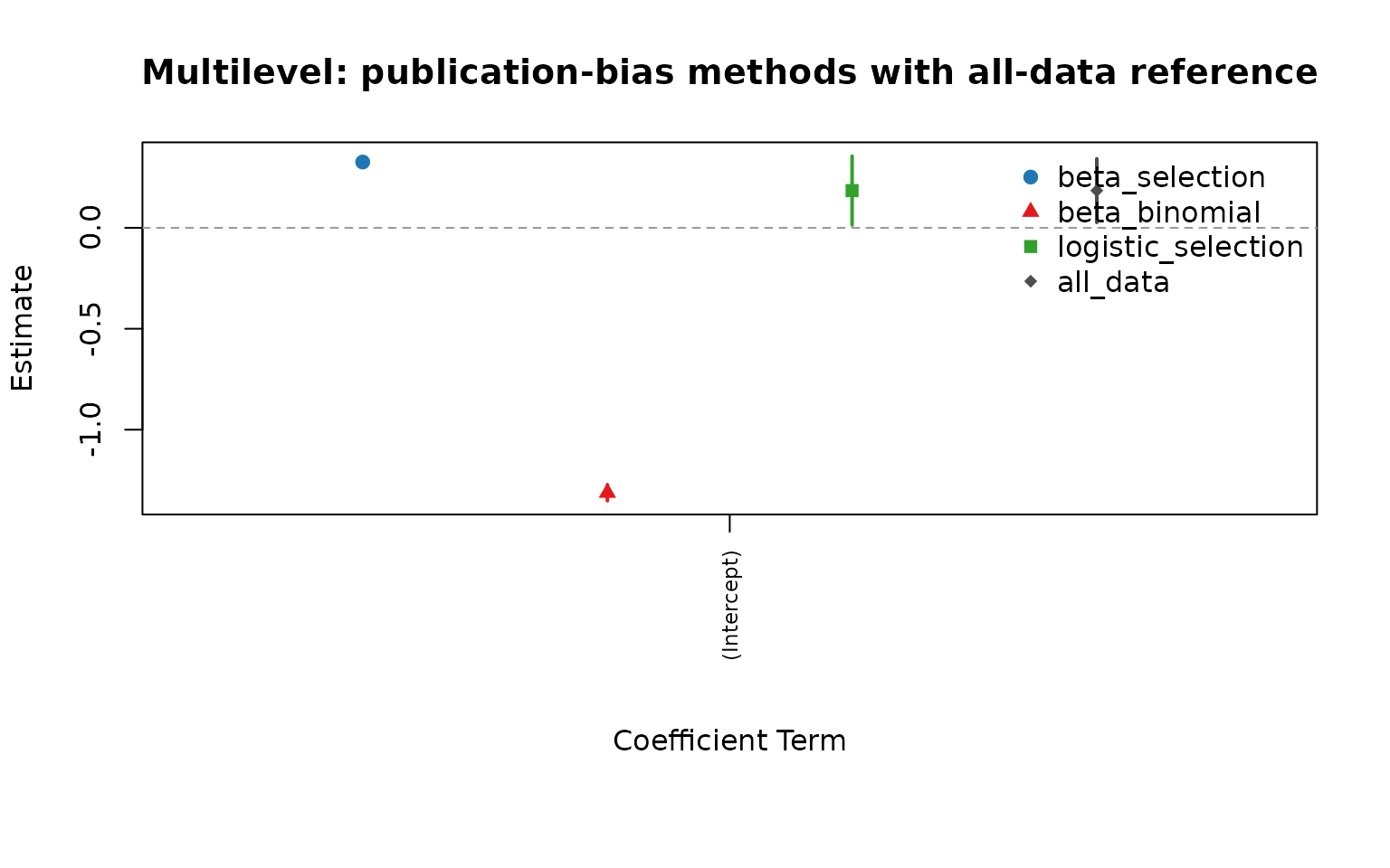
Jackknife version of the multilevel complete-data fit and each publication-bias model:
set.seed(2026)

school_jack <- subset(school, district %in% sort(unique(district))[1:4])

jack_ml_complete <- mars_alt_estimation(
  type = "jackknife",
  data = school_jack,
  formula = effect ~ 1 + (1 | district/study),
  studyID = "district",
  effectID = NULL,
  sample_size = NULL,
  variance = "var",
  varcov_type = "multilevel",
  structure = "multilevel",
  estimation_method = "MLE",
  jackknife_target = "complete_data"
)

jack_ml_beta_selection <- mars_alt_estimation(
  type = "jackknife",
  data = school_jack,
  formula = effect ~ 1 + (1 | district/study),
  studyID = "district",
  effectID = NULL,
  sample_size = NULL,
  variance = "var",
  varcov_type = "multilevel",
  structure = "multilevel",
  estimation_method = "MLE",
  jackknife_target = "beta_selection",
  publication_bias_args = list(
    p_value_tail = "two.sided",
    maxit = 80,
    integration_points = 31
  )
)

jack_ml_beta_binomial <- mars_alt_estimation(
  type = "jackknife",
  data = school_jack,
  formula = effect ~ 1 + (1 | district/study),
  studyID = "district",
  effectID = NULL,
  sample_size = NULL,
  variance = "var",
  varcov_type = "multilevel",
  structure = "multilevel",
  estimation_method = "MLE",
  jackknife_target = "beta_binomial",
  publication_bias_args = list(
    p_value_tail = "two.sided",
    n_bins = 8,
    maxit = 80,
    integration_points = 31
  )
)

jack_ml_logistic <- mars_alt_estimation(
  type = "jackknife",
  data = school_jack,
  formula = effect ~ 1 + (1 | district/study),
  studyID = "district",
  effectID = NULL,
  sample_size = NULL,
  variance = "var",
  varcov_type = "multilevel",
  structure = "multilevel",
  estimation_method = "MLE",
  jackknife_target = "logistic_selection",
  publication_bias_args = list(
    p_value_tail = "two.sided",
    maxit = 80,
    integration_points = 31
  )
)

jack_ml_complete_stats <- compute_alt_stats(jack_ml_complete, type = "jackknife")
jack_ml_beta_selection_stats <- compute_alt_stats(jack_ml_beta_selection, type = "jackknife")
jack_ml_beta_binomial_stats <- compute_alt_stats(jack_ml_beta_binomial, type = "jackknife")
jack_ml_logistic_stats <- compute_alt_stats(jack_ml_logistic, type = "jackknife")

jackknife_compare_ml <- rbind(
  complete_data = extract_alt_interval(jack_ml_complete_stats),
  beta_selection = extract_alt_interval(jack_ml_beta_selection_stats),
  beta_binomial = extract_alt_interval(jack_ml_beta_binomial_stats),
  logistic_selection = extract_alt_interval(jack_ml_logistic_stats)
)

jackknife_compare_ml
The multilevel jackknife illustration uses only the first four top-level clusters so the vignette stays quick to run while still showing the leave-one- cluster-out workflow.
jack_ml_est <- jackknife_compare_ml[, "point_estimate"]
jack_ml_lo <- jackknife_compare_ml[, "ci_lower"]
jack_ml_hi <- jackknife_compare_ml[, "ci_upper"]
xpos_ml <- seq_len(nrow(jackknife_compare_ml))

plot(
  xpos_ml, jack_ml_est,
  ylim = range(c(jack_ml_lo, jack_ml_hi)),
  xaxt = "n", xlab = "", ylab = "Jackknife Estimate",
  pch = 19, col = "#1F78B4",
  main = "Multilevel Jackknife: complete data and publication-bias targets"
)
segments(xpos_ml, jack_ml_lo, xpos_ml, jack_ml_hi, lwd = 2, col = "#1F78B4")
abline(h = 0, lty = 2, col = "gray60")
axis(1, at = xpos_ml, labels = rownames(jackknife_compare_ml), las = 2)
title(xlab = "Jackknife Target", line = 6)
Multivariate Example
becker09 <- na.omit(becker09)

fit_mv <- mars(
  data = becker09,
  studyID = "ID",
  effectID = "numID",
  sample_size = "N",
  effectsize_type = "cor",
  varcov_type = "weighted",
  variable_names = c(
    "Cognitive_Performance",
    "Somatic_Performance",
    "Selfconfidence_Performance",
    "Somatic_Cognitive",
    "Selfconfidence_Cognitive",
    "Selfconfidence_Somatic"
  )
)

summary(fit_mv)
#> Results generated with MARS:v 0.5.2
#> Friday, May 15, 2026
#>
#> Model Type:
#> multivariate
#>
#> Estimation Method:
#> Restricted Maximum Likelihood
#>
#> Model Formula:
#> NULL
#>
#> Data Summary:
#> Number of Effect Sizes: 48
#> Number of Fixed Effects: 6
#> Number of Random Effects: 6
#>
#> Random Components:
#>          ri_1     ri_2     ri_3      ri_4      ri_5       ri_6
#> ri_1  0.13204  0.07630 -0.03144  0.003058 -0.018150  0.0022236
#> ri_2  0.99878  0.04420 -0.01698  0.001532 -0.009861  0.0008355
#> ri_3 -0.42074 -0.39284  0.04229 -0.007313  0.009630 -0.0122546
#> ri_4  0.23176  0.20062 -0.97927  0.001319 -0.001498  0.0022776
#> ri_5 -0.62514 -0.58701  0.58603 -0.516444  0.006384 -0.0024641
#> ri_6  0.09632  0.06256 -0.93797  0.987249 -0.485426  0.0040360
#>
#> Fixed Effects Estimates:
#>  attribute estimate      SE  z_test   p_value   lower     upper
#>          1 -0.09773 0.13777 -0.7093 4.781e-01 -0.3677  0.172299
#>          2 -0.17556 0.08620 -2.0367 4.168e-02 -0.3445 -0.006613
#>          3  0.31868 0.08406  3.7911 1.500e-04  0.1539  0.483438
#>          4  0.52720 0.03335 15.8070 2.785e-56  0.4618  0.592564
#>          5 -0.41756 0.04590 -9.0968 9.305e-20 -0.5075 -0.327591
#>          6 -0.40071 0.04182 -9.5821 9.510e-22 -0.4827 -0.318750
#>
#> Model Fit Statistics:
#>  logLik    Dev   AIC   BIC  AICc
#>   18.63 -37.25 16.75 63.67 29.48
#>
#> Q Error: 230.642 (42), p < 0.0001
#>
#> I2 (General):
#>  names values
#>   ri_1  94.53
#>   ri_2  85.26
#>   ri_3  84.69
#>   ri_4  14.71
#>   ri_5  45.51
#>   ri_6  34.56
#>
#> I2 (Jackson):
#>  names values
#>   ri_1  90.98
#>   ri_2  77.93
#>   ri_3  81.33
#>   ri_4  16.14
#>   ri_5  43.25
#>   ri_6  31.42
#>
#> I2 (Between): 83.393
#>
#> Residual Diagnostics:
#>   n n_finite_raw mean_raw sd_raw   rmse    mae q_pearson mean_abs_studentized
#>  48           48 -0.02155 0.2127 0.2116 0.1646     133.5                1.419
#>  max_abs_studentized prop_abs_studentized_gt2 prop_abs_studentized_gt3
#>                5.006                   0.2708                   0.1042
#>
#> Normality (whitened residuals):                   test n_tested statistic p_value
#>  shapiro_wilk_whitened       48    0.9789  0.5351
#>
#> Heteroscedasticity trend (|raw residual| ~ fitted):   n corr_abs_raw_fitted     slope p_value
#>  48           -0.002893 -0.001091  0.9844
pb_mv <- publication_bias(
  fit_mv,
  method = "beta_selection",
  p_value_tail = "two.sided",
  maxit = 100,
  integration_points = 31
)

summary(pb_mv)
#> Publication Bias Model (MARS)
#> Method: beta_selection
#> Structure: UN
#> Effects: 48  | Studies: 8
#> P-value tail: two.sided
#> Convergence: 0 - Converged
#> Objective: -16.83
#>
#> Selection Parameters:
#>  parameter estimate
#>      alpha   1.0114
#>       beta   0.9479
#>
#> Selection Weight Profile (p-value grid):
#>           model p_value weight
#>  beta_selection  0.0100 0.9493
#>  beta_selection  0.1189 0.9825
#>  beta_selection  0.2278 0.9966
#>  beta_selection  0.3367 1.0090
#>  beta_selection  0.4456 1.0217
#>  beta_selection  0.5544 1.0360
#>  beta_selection  0.6633 1.0534
#>  beta_selection  0.7722 1.0769
#>  beta_selection  0.8811 1.1157
#>  beta_selection  0.9900 1.2710
#>
#> Bias-Adjusted Coefficients:
#>                       term estimate std_error z_value p_value
#>  factor(data[[effectID]])1  -0.1235   14.6343 -0.0084  0.9933
#>  factor(data[[effectID]])2  -0.2511   10.8979 -0.0230  0.9816
#>  factor(data[[effectID]])3   0.3092    3.3025  0.0936  0.9254
#>  factor(data[[effectID]])4   0.5153    6.0255  0.0855  0.9318
#>  factor(data[[effectID]])5  -0.4174    5.4063 -0.0772  0.9385
#>  factor(data[[effectID]])6  -0.4235    2.8873 -0.1467  0.8834
#>
#> Adjusted vs Unadjusted Summary:
#>                       term unadjusted_estimate unadjusted_se
#>  factor(data[[effectID]])1             -0.0977        0.1378
#>  factor(data[[effectID]])2             -0.1756        0.0862
#>  factor(data[[effectID]])3              0.3187        0.0841
#>  factor(data[[effectID]])4              0.5272        0.0334
#>  factor(data[[effectID]])5             -0.4176        0.0459
#>  factor(data[[effectID]])6             -0.4007        0.0418
#>  unadjusted_ci_lower unadjusted_ci_upper estimate std_error adjusted_ci_lower
#>              -0.3678              0.1723  -0.1235   14.6343          -28.8066
#>              -0.3445             -0.0066  -0.2511   10.8979          -21.6111
#>               0.1539              0.4834   0.3092    3.3025           -6.1636
#>               0.4618              0.5926   0.5153    6.0255          -11.2947
#>              -0.5075             -0.3276  -0.4174    5.4063          -11.0137
#>              -0.4827             -0.3187  -0.4235    2.8873           -6.0826
#>  adjusted_ci_upper estimate_diff percent_change direction_changed ci_overlap
#>            28.5596       -0.0258       -26.3896             FALSE       TRUE
#>            21.1088       -0.0756       -43.0508             FALSE       TRUE
#>             6.7821       -0.0094        -2.9631             FALSE       TRUE
#>            12.3253       -0.0119        -2.2526             FALSE       TRUE
#>            10.1789        0.0001         0.0357             FALSE       TRUE
#>             5.2355       -0.0228        -5.6967             FALSE       TRUE
#>
#> Small-Study Effects Check (Egger-type):
#> Model: SND ~ precision
#> Method: Egger-type small-study-effects regression with study-cluster robust SE (CR1)
#> Intercept: -3.8099 SE: 1.2322 t: -3.092 df: 7 p: 0.0175
#>
#> SE note:
#> SE rule: reported SEs use the larger of the Hessian-based and OPG-based values when both are finite, otherwise the finite one. Covariance structure: used the fitted MARS within/between-study covariance blocks directly for the publication-bias likelihood.
pb_mv_bb <- publication_bias(
  fit_mv,
  method = "beta_binomial",
  n_bins = 8,
  p_value_tail = "two.sided",
  maxit = 100,
  integration_points = 31
)

summary(pb_mv_bb)
#> Publication Bias Model (MARS)
#> Method: beta_binomial
#> Structure: UN
#> Effects: 48  | Studies: 8
#> P-value tail: two.sided
#> Convergence: 0 - Converged
#> Objective: -17.59
#>
#> Selection Parameters:
#>  parameter estimate
#>      alpha   1.5143
#>       beta   1.4745
#>     n_bins   8.0000
#>
#> Selection Weight Profile (bin probabilities):
#>  bin p_lower p_upper weight
#>    1   0.000   0.125 0.0841
#>    2   0.125   0.250 0.1192
#>    3   0.250   0.375 0.1389
#>    4   0.375   0.500 0.1486
#>    5   0.500   0.625 0.1499
#>    6   0.625   0.750 0.1428
#>    7   0.750   0.875 0.1253
#>    8   0.875   1.000 0.0912
#>
#> Bias-Adjusted Coefficients:
#>                       term estimate std_error z_value p_value
#>  factor(data[[effectID]])1  -0.1111    0.2607 -0.4263  0.6699
#>  factor(data[[effectID]])2  -0.2491    0.0691 -3.6043  0.0003
#>  factor(data[[effectID]])3   0.3059    0.0907  3.3742  0.0007
#>  factor(data[[effectID]])4   0.5172    0.4988  1.0369  0.2998
#>  factor(data[[effectID]])5  -0.4182    0.2237 -1.8696  0.0615
#>  factor(data[[effectID]])6  -0.4240    0.2348 -1.8058  0.0710
#>
#> Adjusted vs Unadjusted Summary:
#>                       term unadjusted_estimate unadjusted_se
#>  factor(data[[effectID]])1             -0.0977        0.1378
#>  factor(data[[effectID]])2             -0.1756        0.0862
#>  factor(data[[effectID]])3              0.3187        0.0841
#>  factor(data[[effectID]])4              0.5272        0.0334
#>  factor(data[[effectID]])5             -0.4176        0.0459
#>  factor(data[[effectID]])6             -0.4007        0.0418
#>  unadjusted_ci_lower unadjusted_ci_upper estimate std_error adjusted_ci_lower
#>              -0.3678              0.1723  -0.1111    0.2607           -0.6222
#>              -0.3445             -0.0066  -0.2491    0.0691           -0.3845
#>               0.1539              0.4834   0.3059    0.0907            0.1282
#>               0.4618              0.5926   0.5172    0.4988           -0.4605
#>              -0.5075             -0.3276  -0.4182    0.2237           -0.8567
#>              -0.4827             -0.3187  -0.4240    0.2348           -0.8841
#>  adjusted_ci_upper estimate_diff percent_change direction_changed ci_overlap
#>             0.3999       -0.0134       -13.7323             FALSE       TRUE
#>            -0.1136       -0.0735       -41.8828             FALSE       TRUE
#>             0.4836       -0.0128        -4.0076             FALSE       TRUE
#>             1.4949       -0.0100        -1.8977             FALSE       TRUE
#>             0.0202       -0.0007        -0.1594             FALSE       TRUE
#>             0.0362       -0.0232        -5.8017             FALSE       TRUE
#>
#> Small-Study Effects Check (Egger-type):
#> Model: SND ~ precision
#> Method: Egger-type small-study-effects regression with study-cluster robust SE (CR1)
#> Intercept: -3.8099 SE: 1.2322 t: -3.092 df: 7 p: 0.0175
#>
#> SE note:
#> SE rule: reported SEs use the larger of the Hessian-based and OPG-based values when both are finite, otherwise the finite one. Covariance structure: used the fitted MARS within/between-study covariance blocks directly for the publication-bias likelihood. beta_binomial uses discretized p-value bins; coefficient magnitudes can differ materially from beta_selection.
pb_mv_logit <- publication_bias(
  fit_mv,
  method = "logistic_selection",
  p_value_tail = "two.sided",
  maxit = 100,
  integration_points = 31
)

summary(pb_mv_logit)
#> Publication Bias Model (MARS)
#> Method: logistic_selection
#> Structure: UN
#> Effects: 48  | Studies: 8
#> P-value tail: two.sided
#> Convergence: 0 - Converged
#> Objective: -16.75
#>
#> Selection Parameters:
#>        parameter estimate
#>  logit_intercept   2.8831
#>      logit_slope  21.4511
#>
#> Selection Weight Profile (p-value grid):
#>               model p_value weight
#>  logistic_selection  0.0100 1.0000
#>  logistic_selection  0.1189 1.0000
#>  logistic_selection  0.2278 1.0000
#>  logistic_selection  0.3367 1.0000
#>  logistic_selection  0.4456 1.0000
#>  logistic_selection  0.5544 1.0000
#>  logistic_selection  0.6633 1.0000
#>  logistic_selection  0.7722 0.9998
#>  logistic_selection  0.8811 0.9963
#>  logistic_selection  0.9900 0.9568
#>
#> Bias-Adjusted Coefficients:
#>                       term estimate std_error z_value p_value
#>  factor(data[[effectID]])1  -0.0974    0.2440 -0.3992  0.6897
#>  factor(data[[effectID]])2  -0.2345    0.1673 -1.4017  0.1610
#>  factor(data[[effectID]])3   0.2971    0.1265  2.3487  0.0188
#>  factor(data[[effectID]])4   0.5148    0.0671  7.6661  0.0000
#>  factor(data[[effectID]])5  -0.4170    0.0843 -4.9466  0.0000
#>  factor(data[[effectID]])6  -0.4183    0.0630 -6.6361  0.0000
#>
#> Adjusted vs Unadjusted Summary:
#>                       term unadjusted_estimate unadjusted_se
#>  factor(data[[effectID]])1             -0.0977        0.1378
#>  factor(data[[effectID]])2             -0.1756        0.0862
#>  factor(data[[effectID]])3              0.3187        0.0841
#>  factor(data[[effectID]])4              0.5272        0.0334
#>  factor(data[[effectID]])5             -0.4176        0.0459
#>  factor(data[[effectID]])6             -0.4007        0.0418
#>  unadjusted_ci_lower unadjusted_ci_upper estimate std_error adjusted_ci_lower
#>              -0.3678              0.1723  -0.0974    0.2440           -0.5756
#>              -0.3445             -0.0066  -0.2345    0.1673           -0.5625
#>               0.1539              0.4834   0.2971    0.1265            0.0492
#>               0.4618              0.5926   0.5148    0.0671            0.3832
#>              -0.5075             -0.3276  -0.4170    0.0843           -0.5823
#>              -0.4827             -0.3187  -0.4183    0.0630           -0.5418
#>  adjusted_ci_upper estimate_diff percent_change direction_changed ci_overlap
#>             0.3808        0.0003         0.3268             FALSE       TRUE
#>             0.0934       -0.0590       -33.6036             FALSE       TRUE
#>             0.5451       -0.0215        -6.7566             FALSE       TRUE
#>             0.6464       -0.0124        -2.3555             FALSE       TRUE
#>            -0.2518        0.0005         0.1270             FALSE       TRUE
#>            -0.2947       -0.0176        -4.3799             FALSE       TRUE
#>
#> Small-Study Effects Check (Egger-type):
#> Model: SND ~ precision
#> Method: Egger-type small-study-effects regression with study-cluster robust SE (CR1)
#> Intercept: -3.8099 SE: 1.2322 t: -3.092 df: 7 p: 0.0175
#>
#> SE note:
#> SE rule: reported SEs use the larger of the Hessian-based and OPG-based values when both are finite, otherwise the finite one. Covariance structure: used the fitted MARS within/between-study covariance blocks directly for the publication-bias likelihood.
Multivariate coefficients with standard errors:
pb_mv$covariance_mode
#> [1] "fixed_mars_structure"
pb_mv$covariance_structure
#> $structure
#> [1] "UN"
#>
#> $Tau
#>              [,1]          [,2]         [,3]         [,4]         [,5]
#> [1,]  0.132040025  0.0763014664 -0.031441429  0.003058166 -0.018150222
#> [2,]  0.076301466  0.0441998006 -0.016984791  0.001531606 -0.009860779
#> [3,] -0.031441429 -0.0169847911  0.042292885 -0.007313107  0.009629524
#> [4,]  0.003058166  0.0015316061 -0.007313107  0.001318666 -0.001498453
#> [5,] -0.018150222 -0.0098607790  0.009629524 -0.001498453  0.006384168
#> [6,]  0.002223569  0.0008355477 -0.012254561  0.002277566 -0.002464062
#>               [,6]
#> [1,]  0.0022235691
#> [2,]  0.0008355477
#> [3,] -0.0122545613
#> [4,]  0.0022775661
#> [5,] -0.0024640625
#> [6,]  0.0040360241
pb_mv$coefficients
#>                        term   estimate std_error      z_value   p_value
#> 1 factor(data[[effectID]])1 -0.1235143 14.634251 -0.008440084 0.9932659
#> 2 factor(data[[effectID]])2 -0.2511335 10.897949 -0.023044110 0.9816151
#> 3 factor(data[[effectID]])3  0.3092381  3.302479  0.093638194 0.9253966
#> 4 factor(data[[effectID]])4  0.5153197  6.025506  0.085523056 0.9318456
#> 5 factor(data[[effectID]])5 -0.4174073  5.406261 -0.077208142 0.9384580
#> 6 factor(data[[effectID]])6 -0.4235416  2.887272 -0.146692669 0.8833746
pb_mv_bb$coefficients
#>                        term   estimate  std_error    z_value      p_value
#> 1 factor(data[[effectID]])1 -0.1111449 0.26074401 -0.4262606 0.6699179282
#> 2 factor(data[[effectID]])2 -0.2490830 0.06910738 -3.6042898 0.0003130077
#> 3 factor(data[[effectID]])3  0.3059095 0.09066155  3.3741922 0.0007403264
#> 4 factor(data[[effectID]])4  0.5171911 0.49880619  1.0368579 0.2998020984
#> 5 factor(data[[effectID]])5 -0.4182222 0.22369983 -1.8695689 0.0615437017
#> 6 factor(data[[effectID]])6 -0.4239621 0.23478051 -1.8057805 0.0709526289
pb_mv_logit$coefficients
#>                        term   estimate  std_error    z_value      p_value
#> 1 factor(data[[effectID]])1 -0.0974057 0.24397507 -0.3992445 6.897131e-01
#> 2 factor(data[[effectID]])2 -0.2345485 0.16733216 -1.4016944 1.610065e-01
#> 3 factor(data[[effectID]])3  0.2971491 0.12651639  2.3487004 1.883906e-02
#> 4 factor(data[[effectID]])4  0.5147775 0.06714979  7.6661065 1.772960e-14
#> 5 factor(data[[effectID]])5 -0.4170261 0.08430487 -4.9466427 7.550438e-07
#> 6 factor(data[[effectID]])6 -0.4182650 0.06302876 -6.6360968 3.220983e-11
The same idea applies to multivariate fits: the publication-bias
likelihood is evaluated using the fitted MARS within-study covariance
blocks and the fitted between-study Tau matrix, rather than
replacing them with a single scalar heterogeneity term.
ref_mv <- extract_full_data_coefficients(fit_mv)
cmp_mv <- compare_pub_bias_3(pb_mv, pb_mv_bb, pb_mv_logit, ref = ref_mv)
cmp_mv
#>                        term estimate_beta_selection se_beta_selection
#> 1 factor(data[[effectID]])1              -0.1235143         14.634251
#> 2 factor(data[[effectID]])2              -0.2511335         10.897949
#> 3 factor(data[[effectID]])3               0.3092381          3.302479
#> 4 factor(data[[effectID]])4               0.5153197          6.025506
#> 5 factor(data[[effectID]])5              -0.4174073          5.406261
#> 6 factor(data[[effectID]])6              -0.4235416          2.887272
#>   estimate_beta_binomial se_beta_binomial estimate_logistic_selection
#> 1             -0.1111449       0.26074401                  -0.0974057
#> 2             -0.2490830       0.06910738                  -0.2345485
#> 3              0.3059095       0.09066155                   0.2971491
#> 4              0.5171911       0.49880619                   0.5147775
#> 5             -0.4182222       0.22369983                  -0.4170261
#> 6             -0.4239621       0.23478051                  -0.4182650
#>   se_logistic_selection estimate_all_data se_all_data
#> 1            0.24397507       -0.09772505  0.13776971
#> 2            0.16733216       -0.17555552  0.08619682
#> 3            0.12651639        0.31868112  0.08406129
#> 4            0.06714979        0.52719552  0.03335209
#> 5            0.08430487       -0.41755660  0.04590156
#> 6            0.06302876       -0.40071392  0.04181907
plot_pub_bias_compare_3(cmp_mv, main = "Multivariate: publication-bias methods with all-data reference")
Jackknife version of the multivariate complete-data fit and each publication-bias model:
set.seed(2026)

becker09_jack <- becker09[seq_len(min(6, nrow(becker09))), , drop = FALSE]

jack_mv_complete <- mars_alt_estimation(
  type = "jackknife",
  data = becker09_jack,
  studyID = "ID",
  effectID = "numID",
  sample_size = "N",
  effectsize_type = "cor",
  varcov_type = "weighted",
  variable_names = c(
    "Cognitive_Performance",
    "Somatic_Performance",
    "Selfconfidence_Performance",
    "Somatic_Cognitive",
    "Selfconfidence_Cognitive",
    "Selfconfidence_Somatic"
  ),
  structure = "UN",
  estimation_method = "MLE",
  jackknife_target = "complete_data"
)

jack_mv_beta_selection <- mars_alt_estimation(
  type = "jackknife",
  data = becker09_jack,
  studyID = "ID",
  effectID = "numID",
  sample_size = "N",
  effectsize_type = "cor",
  varcov_type = "weighted",
  variable_names = c(
    "Cognitive_Performance",
    "Somatic_Performance",
    "Selfconfidence_Performance",
    "Somatic_Cognitive",
    "Selfconfidence_Cognitive",
    "Selfconfidence_Somatic"
  ),
  structure = "UN",
  estimation_method = "MLE",
  jackknife_target = "beta_selection",
  publication_bias_args = list(
    p_value_tail = "two.sided",
    maxit = 80,
    integration_points = 31
  )
)

jack_mv_beta_binomial <- mars_alt_estimation(
  type = "jackknife",
  data = becker09_jack,
  studyID = "ID",
  effectID = "numID",
  sample_size = "N",
  effectsize_type = "cor",
  varcov_type = "weighted",
  variable_names = c(
    "Cognitive_Performance",
    "Somatic_Performance",
    "Selfconfidence_Performance",
    "Somatic_Cognitive",
    "Selfconfidence_Cognitive",
    "Selfconfidence_Somatic"
  ),
  structure = "UN",
  estimation_method = "MLE",
  jackknife_target = "beta_binomial",
  publication_bias_args = list(
    p_value_tail = "two.sided",
    n_bins = 8,
    maxit = 80,
    integration_points = 31
  )
)

jack_mv_logistic <- mars_alt_estimation(
  type = "jackknife",
  data = becker09_jack,
  studyID = "ID",
  effectID = "numID",
  sample_size = "N",
  effectsize_type = "cor",
  varcov_type = "weighted",
  variable_names = c(
    "Cognitive_Performance",
    "Somatic_Performance",
    "Selfconfidence_Performance",
    "Somatic_Cognitive",
    "Selfconfidence_Cognitive",
    "Selfconfidence_Somatic"
  ),
  structure = "UN",
  estimation_method = "MLE",
  jackknife_target = "logistic_selection",
  publication_bias_args = list(
    p_value_tail = "two.sided",
    maxit = 80,
    integration_points = 31
  )
)

jack_mv_complete_stats <- compute_alt_stats(jack_mv_complete, type = "jackknife")
jack_mv_beta_selection_stats <- compute_alt_stats(jack_mv_beta_selection, type = "jackknife")
jack_mv_beta_binomial_stats <- compute_alt_stats(jack_mv_beta_binomial, type = "jackknife")
jack_mv_logistic_stats <- compute_alt_stats(jack_mv_logistic, type = "jackknife")

mv_term <- pb_mv$coefficients$term[1]
jackknife_compare_mv <- rbind(
  complete_data = extract_alt_interval(jack_mv_complete_stats, term = mv_term),
  beta_selection = extract_alt_interval(jack_mv_beta_selection_stats, term = mv_term),
  beta_binomial = extract_alt_interval(jack_mv_beta_binomial_stats, term = mv_term),
  logistic_selection = extract_alt_interval(jack_mv_logistic_stats, term = mv_term)
)

jackknife_compare_mv
The multivariate jackknife illustration also uses a small subset so the chunk demonstrates the interface without dominating vignette runtime.
jack_mv_est <- jackknife_compare_mv[, "point_estimate"]
jack_mv_lo <- jackknife_compare_mv[, "ci_lower"]
jack_mv_hi <- jackknife_compare_mv[, "ci_upper"]
xpos_mv <- seq_len(nrow(jackknife_compare_mv))

plot(
  xpos_mv, jack_mv_est,
  ylim = range(c(jack_mv_lo, jack_mv_hi)),
  xaxt = "n", xlab = "", ylab = "Jackknife Estimate",
  pch = 19, col = "#1F78B4",
  main = paste("Multivariate Jackknife for", mv_term)
)
segments(xpos_mv, jack_mv_lo, xpos_mv, jack_mv_hi, lwd = 2, col = "#1F78B4")
abline(h = 0, lty = 2, col = "gray60")
axis(1, at = xpos_mv, labels = rownames(jackknife_compare_mv), las = 2)
title(xlab = "Jackknife Target", line = 6)
Method comparison note: - beta_selection and
beta_binomial use different selection-function
parameterizations. - Coefficients and SEs can differ materially,
especially when beta_binomial uses coarse binning or when
Hessian diagnostics indicate weak identifiability. - The
all_data reference intervals come from the original MARS
fit, while publication-bias intervals come from the publication-bias
likelihood with the conservative Hessian-versus-OPG SE rule. - In
multilevel and multivariate settings, publication-bias fits now retain
the fitted MARS covariance structure through
covariance_mode = "fixed_mars_structure".
The same publication-bias interface can be used across univariate,
multilevel, and multivariate mars objects, and both methods
support funnel plotting.