Residual and Influence Diagnostics with MARS
mars authors
2026-05-15
Residual-Diagnostics-Workflow.RmdThis vignette demonstrates residual and influence diagnostics for:
- Univariate models
- Multilevel models
- Multivariate models
using the mars package functions:
residuals(fit, type = ...)residual_diagnostics(fit)influence_diagnostics(fit)
library(mars)The package includes plot_residual_panel() for a compact
three-panel diagnostic plot.
Univariate Example
fit_uni <- mars(
  formula = yi ~ 1,
  data = bcg,
  studyID = "trial",
  variance = "vi",
  varcov_type = "univariate",
  structure = "univariate",
  estimation_method = "MLE"
)

summary(fit_uni)
#> Results generated with MARS:v 0.5.2
#> Friday, May 15, 2026
#>
#> Model Type:
#> univariate
#>
#> Estimation Method:
#> Maximum Likelihood
#>
#> Model Formula:
#> yi ~ 1
#>
#> Data Summary:
#> Number of Effect Sizes: 13
#> Number of Fixed Effects: 1
#> Number of Random Effects: 1
#>
#> Random Components:
#>       term  var     SD
#>  intercept 0.28 0.5292
#>
#> Fixed Effects Estimates:
#>    attribute estimate     SE z_test   p_value  lower   upper
#>  (Intercept)  -0.7112 0.1719 -4.137 3.513e-05 -1.048 -0.3743
#>
#> Model Fit Statistics:
#>  logLik   Dev   AIC   BIC AICc
#>  -12.67 31.33 29.33 30.46 37.9
#>
#> Q Error: 152.233 (12), p < 0.0001
#>
#> I2 (General): 92.03957
#>
#> Residual Diagnostics:
#>   n n_finite_raw mean_raw sd_raw   rmse    mae q_pearson mean_abs_studentized
#>  13           13 -0.02945 0.6938 0.6672 0.5958     13.16               0.9527
#>  max_abs_studentized prop_abs_studentized_gt2 prop_abs_studentized_gt3
#>                1.434                        0                        0
#>
#> Normality (whitened residuals):                   test n_tested statistic p_value
#>  shapiro_wilk_whitened       13     0.886 0.08592
#>
#> Heteroscedasticity trend (|raw residual| ~ fitted):   n corr_abs_raw_fitted slope p_value
#>  13                  NA    NA      NA
Residual vectors:
head(residuals(fit_uni, type = "raw"))
#> [1] -0.17811220 -0.87418952 -0.63687401 -0.73035205  0.49365181 -0.07491645
head(residuals(fit_uni, type = "pearson"))
#> [1] -0.2288738 -1.2689295 -0.7637257 -1.3333495  0.8577297 -0.1398577
head(residuals(fit_uni, type = "studentized"))
#> [1] -0.2346703 -1.3103761 -0.7804878 -1.4042904  0.8987531 -0.1476677
head(residuals(fit_uni, type = "whitened"))
#> [1] -0.2288738 -1.2689295 -0.7637257 -1.3333495  0.8577297 -0.1398577
Diagnostics summary:
rd_uni <- residual_diagnostics(fit_uni)
rd_uni$summary
#>    n n_finite_raw    mean_raw   sd_raw      rmse      mae q_pearson
#> 1 13           13 -0.02945125 0.693805 0.6672366 0.595824   13.1642
#>   mean_abs_studentized max_abs_studentized prop_abs_studentized_gt2
#> 1            0.9526839            1.433625                        0
#>   prop_abs_studentized_gt3
#> 1                        0
rd_uni$normality
#>                    test n_tested statistic   p_value
#> 1 shapiro_wilk_whitened       13 0.8859613 0.0859246
rd_uni$heteroscedasticity
#>    n corr_abs_raw_fitted slope p_value
#> 1 13                  NA    NA      NA
Influence summary:
inf_uni <- influence_diagnostics(fit_uni, top_n = 5)
head(inf_uni$influence)
#>   index     fitted         raw studentized   leverage cooks_distance
#> 1     1 -0.7111991 -0.17811220  -0.2346703 0.04879109    0.002824756
#> 2     2 -0.7111991 -0.87418952  -1.3103761 0.06225861    0.114000889
#> 3     3 -0.7111991 -0.63687401  -0.7804878 0.04249163    0.027032924
#> 4     4 -0.7111991 -0.73035205  -1.4042904 0.09848251    0.215426344
#> 5     5 -0.7111991  0.49365181   0.8987531 0.08920621    0.079114458
#> 6     6 -0.7111991 -0.07491645  -0.1476677 0.10298026    0.002503357
#>   influence_score flagged cluster
#> 1      0.05314843   FALSE       1
#> 2      0.33764018   FALSE       2
#> 3      0.16441692   FALSE       3
#> 4      0.46414044   FALSE       4
#> 5      0.28127292   FALSE       5
#> 6      0.05003355   FALSE       6
inf_uni$thresholds
#>    n p cooks_distance  leverage abs_studentized
#> 1 13 1      0.3076923 0.1538462               2
inf_uni$top
#>    index     fitted        raw studentized   leverage cooks_distance
#> 8      8 -0.7111991  0.7231515    1.433625 0.10404783      0.2386818
#> 4      4 -0.7111991 -0.7303521   -1.404290 0.09848251      0.2154263
#> 13    13 -0.7111991  0.6938852    1.223032 0.08408012      0.1373129
#> 10    10 -0.7111991 -0.6601457   -1.160646 0.08369429      0.1230424
#> 2      2 -0.7111991 -0.8741895   -1.310376 0.06225861      0.1140009
#>    influence_score flagged cluster
#> 8        0.4885507   FALSE       8
#> 4        0.4641404   FALSE       4
#> 13       0.3705575   FALSE      13
#> 10       0.3507740   FALSE      10
#> 2        0.3376402   FALSE       2
plot_residual_panel(fit_uni, main_prefix = "Univariate", fitted_jitter = 0.02)
Multilevel Example
fit_ml <- mars(
  formula = effect ~ 1 + (1 | district/study),
  data = school,
  studyID = "district",
  variance = "var",
  varcov_type = "multilevel",
  structure = "multilevel",
  estimation_method = "MLE"
)

summary(fit_ml)
#> Results generated with MARS:v 0.5.2
#> Friday, May 15, 2026
#>
#> Model Type:
#> multilevel
#>
#> Estimation Method:
#> Maximum Likelihood
#>
#> Model Formula:
#> effect ~ 1 + (1 | district/study)
#>
#> Data Summary:
#> Number of Effect Sizes: 56
#> Number of Fixed Effects: 1
#> Number of Random Effects: 2
#>
#> Random Data Summary:
#> Number unique district: 11
#> Number unique study: 56
#>
#> Random Components:
#>      term     var     SD
#>  district 0.05774 0.2403
#>     study 0.03286 0.1813
#>
#> Fixed Effects Estimates:
#>    attribute estimate      SE z_test p_value   lower  upper
#>  (Intercept)   0.1845 0.08048  2.292 0.02191 0.02671 0.3422
#>
#> Model Fit Statistics:
#>  logLik   Dev   AIC   BIC AICc
#>  -8.395 24.79 22.79 28.87 24.5
#>
#> Q Error: 578.864 (55), p < 0.0001
#>
#> I2 (General):
#>     names values
#>  district  92.38
#>     study  87.34
#>
#> I2 (Jackson): 98.69621
#> I2 (Between): 86.3727
#>
#> Residual Diagnostics:
#>   n n_finite_raw mean_raw sd_raw   rmse    mae q_pearson mean_abs_studentized
#>  56           56 -0.06446 0.3258 0.3293 0.2632      96.8                1.065
#>  max_abs_studentized prop_abs_studentized_gt2 prop_abs_studentized_gt3
#>                4.196                   0.1071                  0.03571
#>
#> Normality (whitened residuals):                   test n_tested statistic p_value
#>  shapiro_wilk_whitened       56    0.9555 0.03766
#>
#> Heteroscedasticity trend (|raw residual| ~ fitted):   n corr_abs_raw_fitted slope p_value
#>  56                  NA    NA      NA
Residual diagnostics with cluster-level summaries:
rd_ml <- residual_diagnostics(fit_ml)
rd_ml$summary
#>    n n_finite_raw    mean_raw    sd_raw      rmse       mae q_pearson
#> 1 56           56 -0.06445539 0.3258499 0.3292972 0.2632178  96.79523
#>   mean_abs_studentized max_abs_studentized prop_abs_studentized_gt2
#> 1             1.064823            4.196444                0.1071429
#>   prop_abs_studentized_gt3
#> 1               0.03571429
head(rd_ml$by_cluster)
#>   district  n    mean_raw      rmse mean_abs_studentized q_pearson
#> 1       11  4 -0.30195539 0.3650970            0.7534140  2.811820
#> 2       12  4 -0.08945539 0.2339386            0.6520311  3.617217
#> 3       18  3  0.18887795 0.1999094            0.6839756  1.522650
#> 4       27  4  0.25804461 0.3243544            1.2306973  8.539825
#> 5       56  4 -0.12195539 0.1513006            0.5560039  1.824676
#> 6       58 11 -0.26172811 0.2879608            1.1493145 16.901115
Influence diagnostics with cluster aggregation:
inf_ml <- influence_diagnostics(fit_ml, top_n = 8)
head(inf_ml$influence)
#>   index    fitted         raw studentized   leverage cooks_distance
#> 1     1 0.1844554 -0.36445539  -0.8686214 0.01775366   0.0136373080
#> 2     2 0.1844554 -0.40445539  -0.9639550 0.01775366   0.0167950441
#> 3     3 0.1844554  0.04554461   0.1014940 0.01514379   0.0001583953
#> 4     4 0.1844554 -0.48445539  -1.0795856 0.01514379   0.0179215621
#> 5     5 0.1844554 -0.05445539  -0.2253871 0.02430887   0.0012656409
#> 6     6 0.1844554 -0.44445539  -1.8395701 0.02430887   0.0843111753
#>   influence_score flagged cluster
#> 1      0.11677888   FALSE      11
#> 2      0.12959569   FALSE      11
#> 3      0.01258552   FALSE      11
#> 4      0.13387144   FALSE      11
#> 5      0.03557585   FALSE      12
#> 6      0.29036387    TRUE      12
head(inf_ml$by_cluster)
#>   district  n max_abs_studentized max_leverage   cook_sum   cook_max n_flagged
#> 1       11  4           1.0795856   0.01775366 0.04851231 0.01792156         0
#> 2       12  4           1.8395701   0.02430887 0.09112591 0.08431118         1
#> 3       18  3           0.9849686   0.03537232 0.04377601 0.02836556         0
#> 4       27  4           2.1496261   0.02633070 0.22966122 0.12496166         2
#> 5       56  4           1.1282772   0.02641107 0.04847426 0.03453360         0
#> 6       58 11           2.0187576   0.01123359 0.15388801 0.03330217         1
inf_ml$top
#>    index    fitted        raw studentized   leverage cooks_distance
#> 33    33 0.1844554  1.0055446    4.196444 0.03103164     0.56397255
#> 32    32 0.1844554  0.7955446    3.295059 0.03032420     0.33953866
#> 13    13 0.1844554  0.4655446    2.149626 0.02633070     0.12496166
#> 48    48 0.1844554 -0.7044554   -2.574604 0.01822990     0.12308219
#> 15    15 0.1844554  0.4155446    1.864420 0.02434920     0.08675166
#> 6      6 0.1844554 -0.4444554   -1.839570 0.02430887     0.08431118
#> 43    43 0.1844554  0.4755446    2.113685 0.01657822     0.07531445
#> 52    52 0.1844554 -0.5244554   -1.929236 0.01851989     0.07023077
#>    influence_score flagged cluster
#> 33       0.7509811    TRUE      71
#> 32       0.5826995    TRUE      71
#> 13       0.3534992    TRUE      27
#> 48       0.3508307    TRUE     108
#> 15       0.2945363    TRUE      27
#> 6        0.2903639    TRUE      12
#> 43       0.2744348    TRUE      91
#> 52       0.2650109   FALSE     108
plot_residual_panel(fit_ml, main_prefix = "Multilevel", fitted_jitter = 0.02)
Multivariate Example
fit_mv <- mars(
  data = becker09,
  studyID = "ID",
  effectID = "numID",
  sample_size = "N",
  effectsize_type = "cor",
  varcov_type = "weighted",
  variable_names = c(
    "Cognitive_Performance",
    "Somatic_Performance",
    "Selfconfidence_Performance",
    "Somatic_Cognitive",
    "Selfconfidence_Cognitive",
    "Selfconfidence_Somatic"
  )
)

summary(fit_mv)
#> Results generated with MARS:v 0.5.2
#> Friday, May 15, 2026
#>
#> Model Type:
#> multivariate
#>
#> Estimation Method:
#> Restricted Maximum Likelihood
#>
#> Model Formula:
#> NULL
#>
#> Data Summary:
#> Number of Effect Sizes: 54
#> Number of Fixed Effects: 6
#> Number of Random Effects: 6
#>
#> Random Components:
#>         ri_1     ri_2     ri_3      ri_4      ri_5      ri_6
#> ri_1  0.1221  0.07342 -0.02923  0.002719 -0.015945  0.003653
#> ri_2  0.8992  0.05460 -0.02882  0.003697 -0.012822  0.001786
#> ri_3 -0.3645 -0.53747  0.05266 -0.009075  0.012947 -0.013151
#> ri_4  0.1934  0.39320 -0.98293  0.001619 -0.002136  0.002353
#> ri_5 -0.5668 -0.68157  0.70076 -0.659537  0.006482 -0.002520
#> ri_6  0.1487  0.10871 -0.81499  0.831698 -0.445197  0.004945
#>
#> Fixed Effects Estimates:
#>  attribute estimate      SE  z_test   p_value    lower   upper
#>          1 -0.02286 0.12024 -0.1901 8.492e-01 -0.25853  0.2128
#>          2 -0.06819 0.08607 -0.7923 4.282e-01 -0.23688  0.1005
#>          3  0.23486 0.08614  2.7264 6.403e-03  0.06602  0.4037
#>          4  0.54220 0.03456 15.6895 1.784e-55  0.47447  0.6099
#>          5 -0.44472 0.04717 -9.4278 4.187e-21 -0.53717 -0.3523
#>          6 -0.38870 0.04407 -8.8199 1.145e-18 -0.47507 -0.3023
#>
#> Model Fit Statistics:
#>  logLik    Dev   AIC   BIC  AICc
#>   15.39 -30.79 23.21 73.73 33.98
#>
#> Q Error: 217.704 (48), p < 0.0001
#>
#> I2 (General):
#>  names values
#>   ri_1  92.91
#>   ri_2  85.43
#>   ri_3  84.98
#>   ri_4  14.81
#>   ri_5  41.05
#>   ri_6  34.69
#>
#> I2 (Jackson):
#>  names values
#>   ri_1  89.19
#>   ri_2  79.35
#>   ri_3  82.78
#>   ri_4  17.29
#>   ri_5  39.51
#>   ri_6  33.65
#>
#> I2 (Between): 81.26981
#>
#> Residual Diagnostics:
#>   n n_finite_raw mean_raw sd_raw   rmse   mae q_pearson mean_abs_studentized
#>  54           54 -0.01122 0.2431 0.2411 0.184     109.9                1.217
#>  max_abs_studentized prop_abs_studentized_gt2 prop_abs_studentized_gt3
#>                  4.1                   0.1852                  0.05556
#>
#> Normality (whitened residuals):                   test n_tested statistic p_value
#>  shapiro_wilk_whitened       54    0.9797  0.4891
#>
#> Heteroscedasticity trend (|raw residual| ~ fitted):   n corr_abs_raw_fitted     slope p_value
#>  54           0.0002964 0.0001388  0.9983
Outcome-level residual diagnostics:
rd_mv <- residual_diagnostics(fit_mv)
rd_mv$summary
#>    n n_finite_raw  mean_raw    sd_raw      rmse       mae q_pearson
#> 1 54           54 -0.011217 0.2431376 0.2411368 0.1840274  109.8781
#>   mean_abs_studentized max_abs_studentized prop_abs_studentized_gt2
#> 1             1.216883            4.099539                0.1851852
#>   prop_abs_studentized_gt3
#> 1               0.05555556
head(rd_mv$by_outcome)
#>   numID  n     mean_raw      rmse mean_abs_studentized q_pearson
#> 1     1 10 -0.007139423 0.3669482            1.4940899 27.248239
#> 2     2 10  0.006190537 0.2788446            1.5617825 34.221644
#> 3     3  9 -0.003746967 0.2409277            1.2194742 18.540068
#> 4     4  9 -0.019982101 0.1315502            0.8078973  7.385632
#> 5     5  8  0.002219055 0.1463683            1.0460046 11.179758
#> 6     6  8 -0.050052528 0.1441915            1.0673225 11.302729
Outcome-level influence diagnostics:
inf_mv <- influence_diagnostics(fit_mv, top_n = 10)
head(inf_mv$influence)
#>   index      fitted         raw studentized  leverage cooks_distance
#> 1     1 -0.02286058 -0.52713942  -3.1911778 0.1186167     0.22841875
#> 2     2 -0.06819054 -0.41180946  -4.0995393 0.1628761     0.54498752
#> 3     3  0.23485808  0.42514192   3.3272243 0.1468333     0.31754387
#> 4     4  0.54220432 -0.07220432  -1.3291631 0.2407873     0.09338465
#> 5     5 -0.44471906  0.06471906   0.8577427 0.2138190     0.03334929
#> 6     6 -0.38869747 -0.07130253  -1.0531615 0.2253220     0.05376767
#>   influence_score flagged cluster outcome
#> 1       1.1706889    TRUE       1       1
#> 2       1.8082934    TRUE       1       2
#> 3       1.3803127    TRUE       1       3
#> 4       0.7485372    TRUE       1       4
#> 5       0.4473206   FALSE       1       5
#> 6       0.5679842    TRUE       1       6
head(inf_mv$by_outcome)
#>   numID  n max_abs_studentized max_leverage  cook_sum   cook_max n_flagged
#> 1     1 10            3.191178    0.1186167 0.5895304 0.22841875         3
#> 2     2 10            4.099539    0.1628761 0.9088137 0.54498752         4
#> 3     3  9            3.327224    0.1468333 0.5469411 0.31754387         2
#> 4     4  9            1.726930    0.2407873 0.2020551 0.09338465         1
#> 5     5  8            2.242872    0.2138190 0.3162518 0.10584795         2
#> 6     6  8            2.219610    0.2253220 0.3248226 0.11907408         3
inf_mv$top
#>    index      fitted        raw studentized   leverage cooks_distance
#> 2      2 -0.06819054 -0.4118095   -4.099539 0.16287612      0.5449875
#> 3      3  0.23485808  0.4251419    3.327224 0.14683334      0.3175439
#> 1      1 -0.02286058 -0.5271394   -3.191178 0.11861670      0.2284187
#> 32    32 -0.06819054 -0.3618095   -2.595997 0.09655881      0.1200464
#> 42    42 -0.38869747  0.1186975    1.656690 0.20654264      0.1190741
#> 23    23 -0.06819054  0.3781905    2.579055 0.08993286      0.1095506
#> 31    31 -0.02286058 -0.4971394   -2.398921 0.10235719      0.1093693
#> 7      7 -0.02286058  0.5528606    2.457779 0.09635057      0.1073467
#> 29    29 -0.44471906  0.1547191    1.767094 0.16900934      0.1058480
#> 35    35 -0.44471906  0.2647191    2.242872 0.10265672      0.0959150
#>    influence_score flagged cluster outcome
#> 2        1.8082934    TRUE       1       2
#> 3        1.3803127    TRUE       1       3
#> 1        1.1706889    TRUE       1       1
#> 32       0.8486923    TRUE      26       2
#> 42       0.8452482    TRUE      28       6
#> 23       0.8107427    TRUE      17       2
#> 31       0.8100715    TRUE      26       1
#> 7        0.8025461    TRUE       3       1
#> 29       0.7969239    TRUE      22       5
#> 35       0.7586106    TRUE      26       5
plot_residual_panel(fit_mv, main_prefix = "Multivariate", fitted_jitter = 0.02)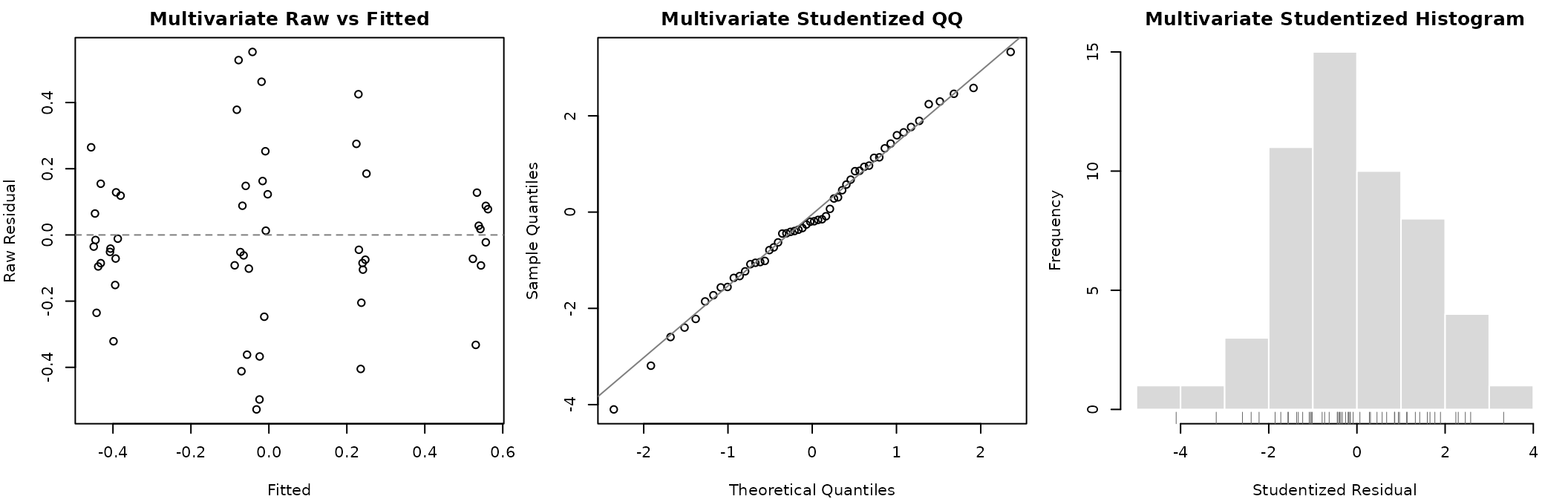
Set fitted_jitter = 0 to keep the original plot, or use
a small positive value to spread overlapping fitted values in the
raw-residual panel. The histogram panel automatically uses
"Sturges" breaks for smaller samples and "FD"
for larger ones, and adds a rug to show the observed residual values
directly.
Practical Interpretation Notes
Use diagnostics as a combined signal:
- Large absolute studentized residuals suggest local model-data misfit.
- Large Cook’s distance and leverage identify influential points.
- Cluster-level aggregation (
by_cluster) helps flag higher-level units that dominate multilevel fits. - Outcome-level aggregation (
by_outcome) helps detect systematic outcome-specific misfit in multivariate analyses.
No single threshold is definitive; use diagnostics with substantive context and sensitivity analyses.