Scale-Location Models with MARS

Scale-location models let the fixed-effect formula describe the mean effect while scale_formula describes heterogeneity on the log scale. This vignette is intentionally small: it shows the core workflow and returned objects without building a full applied analysis.

library(mars)

Univariate Scale-Location Model

The bundled school data contain one effect-size estimate and sampling variance per row. In the model below, effect ~ year is the location model and scale_formula = ~ year lets the between-study standard deviation vary with year.

fit_uni_scale <- mars(
  data = school,
  formula = effect ~ year,
  scale_formula = ~ year,
  studyID = "study",
  variance = "var",
  varcov_type = "univariate",
  structure = "univariate",
  estimation_method = "MLE"
)

summary(fit_uni_scale)
#> Results generated with MARS:v 0.5.2 
#> Friday, May 15, 2026
#> 
#> Model Type: 
#> univariate
#> 
#> Estimation Method: 
#> Maximum Likelihood
#> 
#> Model Formula: 
#> effect ~ year
#> 
#> Scale Formula: 
#> ~year
#> 
#> Data Summary: 
#> Number of Effect Sizes: 56
#> Number of Fixed Effects: 2
#> Number of Random Effects: 3
#> 
#> Random Components: 
#>    term     var     SD
#>     min 0.08569 0.2927
#>  median 0.08627 0.2937
#>     max 0.08825 0.2971
#> 
#> Fixed Effects Estimates: 
#>    attribute   estimate        SE z_test p_value      lower    upper
#>  (Intercept) -12.978322 11.960501 -1.085  0.2779 -36.420473 10.46383
#>         year   0.006584  0.006011  1.095  0.2734  -0.005199  0.01837
#> 
#> 
#> Scale Effects Estimates: 
#>    attribute   estimate SE z_test p_value      lower      upper
#>  (Intercept) -6.185e-07  0   -Inf       0 -6.185e-07 -6.185e-07
#>         year -1.229e-03  0   -Inf       0 -1.229e-03 -1.229e-03
#> 
#> Model Fit Statistics: 
#>  logLik   Dev   AIC   BIC  AICc
#>  -16.69 43.38 41.38 49.48 43.71
#> 
#> Q Error: 550.26 (54), p < 0.0001
#> 
#> I2 (General): 
#>    term values
#>     min  94.62
#>  median  94.65
#>     max  94.77
#> 
#> 
#> Residual Diagnostics: 
#>   n n_finite_raw   mean_raw sd_raw  rmse   mae q_pearson mean_abs_studentized
#>  56           56 -3.659e-07 0.3189 0.316 0.239     27.35               0.5379
#>  max_abs_studentized prop_abs_studentized_gt2 prop_abs_studentized_gt3
#>                2.292                  0.01786                        0
#> 
#> Normality (whitened residuals):                   test n_tested statistic  p_value
#>  shapiro_wilk_whitened       56    0.9317 0.003475
#> 
#> Heteroscedasticity trend (|raw residual| ~ fitted):   n corr_abs_raw_fitted  slope p_value
#>  56              0.1496 0.4664  0.2712

The fitted object stores the scale coefficients and the implied heterogeneity values. For univariate scale-location models, est_values$Tau has one value per effect-size row.

fit_uni_scale$scale_coefficients
#>     attribute      estimate
#> 1 (Intercept) -6.184863e-07
#> 2        year -1.228521e-03
head(fit_uni_scale$est_values$Tau)
#> [1] 0.08825216 0.08825216 0.08825216 0.08825216 0.08685390 0.08685390
range(fit_uni_scale$est_values$Tau)
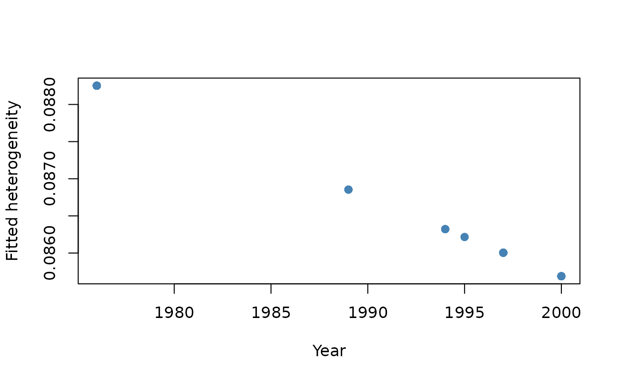
#> [1] 0.08568807 0.08825216

The coefficients are on the log-heterogeneity scale. A simple way to inspect the fitted pattern is to plot Tau against the scale predictor.

plot(
  school$year,
  fit_uni_scale$est_values$Tau,
  xlab = "Year",
  ylab = "Fitted heterogeneity",
  pch = 19,
  col = "steelblue"
)

Multilevel Scale-Location Model

For multilevel models, scale_formula can be a single one-sided formula applied to each random-effect component. Here the scale side is intercept-only, so each component has its own baseline heterogeneity.

fit_ml_scale <- mars(
  data = school,
  formula = effect ~ 1 + (1 | district/study),
  scale_formula = ~ 1,
  studyID = "district",
  variance = "var",
  varcov_type = "multilevel",
  structure = "multilevel",
  estimation_method = "MLE"
)

summary(fit_ml_scale)
#> Results generated with MARS:v 0.5.2 
#> Friday, May 15, 2026
#> 
#> Model Type: 
#> multilevel
#> 
#> Estimation Method: 
#> Maximum Likelihood
#> 
#> Model Formula: 
#> effect ~ 1 + (1 | district/study)
#> 
#> Scale Formula: 
#> ~1
#> 
#> Data Summary: 
#> Number of Effect Sizes: 56
#> Number of Fixed Effects: 1
#> Number of Random Effects: 2
#> 
#> Random Data Summary: 
#> Number unique district: 11 
#> Number unique study: 56
#> 
#> Random Components: 
#>      term     var     SD
#>  district 0.05774 0.2403
#>     study 0.03286 0.1813
#> 
#> Fixed Effects Estimates: 
#>    attribute estimate      SE z_test p_value   lower  upper
#>  (Intercept)   0.1845 0.08048  2.292 0.02191 0.02671 0.3422
#> 
#> 
#> Scale Effects Estimates: 
#>    attribute component estimate     SE  z_test   p_value  lower  upper
#>  (Intercept)  district   -2.852 0.5324  -5.356 8.501e-08 -3.895 -1.808
#>  (Intercept)     study   -3.415 0.3390 -10.076 7.045e-24 -4.080 -2.751
#> 
#> Model Fit Statistics: 
#>  logLik   Dev   AIC   BIC AICc
#>  -8.395 24.79 22.79 28.87 24.5
#> 
#> Q Error: 578.864 (55), p < 0.0001
#> 
#> I2 (General): 
#>     names values
#>  district  92.38
#>     study  87.34
#> 
#> I2 (Jackson): 98.6962
#> I2 (Between): 86.3727
#> 
#> Residual Diagnostics: 
#>   n n_finite_raw mean_raw sd_raw   rmse    mae q_pearson mean_abs_studentized
#>  56           56 -0.06446 0.3258 0.3293 0.2632     96.79                1.065
#>  max_abs_studentized prop_abs_studentized_gt2 prop_abs_studentized_gt3
#>                4.196                   0.1071                  0.03571
#> 
#> Normality (whitened residuals):                   test n_tested statistic p_value
#>  shapiro_wilk_whitened       56    0.9555 0.03766
#> 
#> Heteroscedasticity trend (|raw residual| ~ fitted):   n corr_abs_raw_fitted slope p_value
#>  56                  NA    NA      NA

The returned scale table identifies which random-effect component each scale coefficient belongs to. Tau_by_study gives the fitted component-specific heterogeneity values by top-level cluster.

fit_ml_scale$scale_coefficients
#>     attribute component  estimate
#> 1 (Intercept)  district -2.851841
#> 2 (Intercept)     study -3.415352
head(fit_ml_scale$est_values$Tau_by_study)
#>        district      study
#> [1,] 0.05773792 0.03286485
#> [2,] 0.05773792 0.03286485
#> [3,] 0.05773792 0.03286485
#> [4,] 0.05773792 0.03286485
#> [5,] 0.05773792 0.03286485
#> [6,] 0.05773792 0.03286485

Component-Specific Scale Formulas

Multilevel scale models also accept a named list of formulas, one per random-effect component. Scale predictors must be invariant within the top-level studyID cluster. The code below creates a district-level version of year and uses it only for the study component.

school2 <- school
school2$district_year <- ave(school2$year, school2$district, FUN = min)

fit_component_scale <- mars(
  data = school2,
  formula = effect ~ 1 + (1 | district/study),
  scale_formula = list(
    district = ~ 1,
    study = ~ 1 + district_year
  ),
  studyID = "district",
  variance = "var",
  varcov_type = "multilevel",
  structure = "multilevel",
  estimation_method = "MLE"
)

fit_component_scale$scale_coefficients
head(fit_component_scale$est_values$Tau_by_study)

In short, scale_formula is the scale-side analogue of the location formula: use the main formula for average effects and scale_formula for modeled heterogeneity.

mars authors

2026-05-15

Univariate Scale-Location Model

Multilevel Scale-Location Model

Component-Specific Scale Formulas