Profile Likelihood with MARS

This vignette shows the low-runtime profile-likelihood helpers in mars. Profile likelihoods are useful when Wald intervals for variance components are too symmetric or too dependent on the local curvature at the optimum. The profile plots use the fitted model objective on a deviance-like scale, so lower values indicate better fit and chi-square cutoffs can be drawn above the fitted minimum.

Interpreting Profile Likelihoods

A profile likelihood plot is analogous to plotting the likelihood directly, but on the optimizer’s deviance-scale metric. In this package, lower values indicate better fit. For ordinary mars models, the objective is equivalent to -2 log L up to constants that do not change across the profile; for publication-bias profiles, the same -2 log L scaling is used.

For a one-dimensional profile:

The x-axis is the value of the parameter being held fixed.
The y-axis is the deviance-scale objective after all other parameters have been re-optimized.
The bottom of the curve is the best-supported value on the grid.
The horizontal cutoff line is the fitted minimum plus qchisq(level, df = 1). For a 95% profile interval, this is approximately 3.84 above the minimum.

For a two-dimensional profile surface, the x- and y-axes are two parameters held fixed together. Each contour shows how much worse the best possible model fit is after all remaining parameters are allowed to adapt. The highlighted cutoff contour uses qchisq(level, df = 2) above the fitted minimum and can be read as an approximate joint confidence region for the parameter pair.

library(mars)

Fit a Small Model

We use the bundled bcg data and fit a univariate meta-regression. The examples below intentionally use small grids so the vignette compiles quickly.

fit_bcg <- mars(
  formula = yi ~ year,
  data = bcg,
  studyID = "trial",
  variance = "vi",
  varcov_type = "univariate",
  structure = "univariate",
  estimation_method = "MLE"
)

summary(fit_bcg)
#> Results generated with MARS:v 0.5.2 
#> Friday, May 15, 2026
#> 
#> Model Type: 
#> univariate
#> 
#> Estimation Method: 
#> Maximum Likelihood
#> 
#> Model Formula: 
#> yi ~ year
#> 
#> Data Summary: 
#> Number of Effect Sizes: 13
#> Number of Fixed Effects: 2
#> Number of Random Effects: 1
#> 
#> Random Components: 
#>       term    var    SD
#>  intercept 0.2819 0.531
#> 
#> Fixed Effects Estimates: 
#>    attribute estimate       SE z_test p_value      lower    upper
#>  (Intercept) -53.2412 32.70445 -1.628  0.1035 -117.34072 10.85839
#>         year   0.0267  0.01662  1.606  0.1082   -0.00588  0.05928
#> 
#> Model Fit Statistics: 
#>  logLik  Dev  AIC  BIC AICc
#>   -12.7 35.4 31.4 33.1 53.8
#> 
#> Q Error: 100.178 (11), p < 0.0001
#> 
#> I2 (General): 89.2357
#> 
#> Residual Diagnostics: 
#>   n n_finite_raw mean_raw sd_raw   rmse    mae q_pearson mean_abs_studentized
#>  13           13 0.006114 0.6259 0.6013 0.5193     10.52               0.8597
#>  max_abs_studentized prop_abs_studentized_gt2 prop_abs_studentized_gt3
#>                1.974                        0                        0
#> 
#> Normality (whitened residuals):                   test n_tested statistic p_value
#>  shapiro_wilk_whitened       13    0.8975  0.1237
#> 
#> Heteroscedasticity trend (|raw residual| ~ fitted):   n corr_abs_raw_fitted  slope p_value
#>  13              0.3116 0.3369     0.3

One-Dimensional Profiles

profile_likelihood() can profile fixed-effect parameters by name and random effect parameters as tau1, tau2, and so on.

pr <- profile_likelihood(
  fit_bcg,
  parameters = c("year", "tau1"),
  n_points = 5,
  span = 2
)

pr$summary
#>   parameter parameter_index           mle   cutoff  ci_lower   ci_upper
#> 1      year               2 -0.0003590629 5.349309 -0.053254 0.05430397
#> 2      tau1               3  0.2819106893 5.349309        NA 0.98583762

Each profiled parameter has a data frame containing the fixed grid value, the conditional deviance-scale objective value, and optimizer convergence status. The objective column is the plotted outcome; it is not the original effect-size outcome variable.

pr$profiles$year
#>   parameter parameter_index parameter_value objective converged
#> 1      year               2          -2e+00 92.531406      TRUE
#> 2      year               2          -1e+00 74.888767      TRUE
#> 3      year               2           2e-08  1.437747      TRUE
#> 4      year               2           2e-08  1.437747     FALSE
#> 5      year               2           1e+00 73.468648      TRUE
#> 6      year               2           2e+00 91.819622      TRUE
pr$profiles$tau1
#>   parameter parameter_index parameter_value objective converged
#> 1      tau1               3       0.1409553 -0.814914      TRUE
#> 2      tau1               3       0.2819107 -1.142022      TRUE
#> 3      tau1               3       0.2827391 -1.136381      TRUE
#> 4      tau1               3       0.5671398  1.619323      TRUE
#> 5      tau1               3       1.1376125  6.701402      TRUE
#> 6      tau1               3       2.2819107 13.415105      TRUE

The plot method draws a profile curve and invisibly returns the data frame used for the plot.

plot(pr, parameter = "year")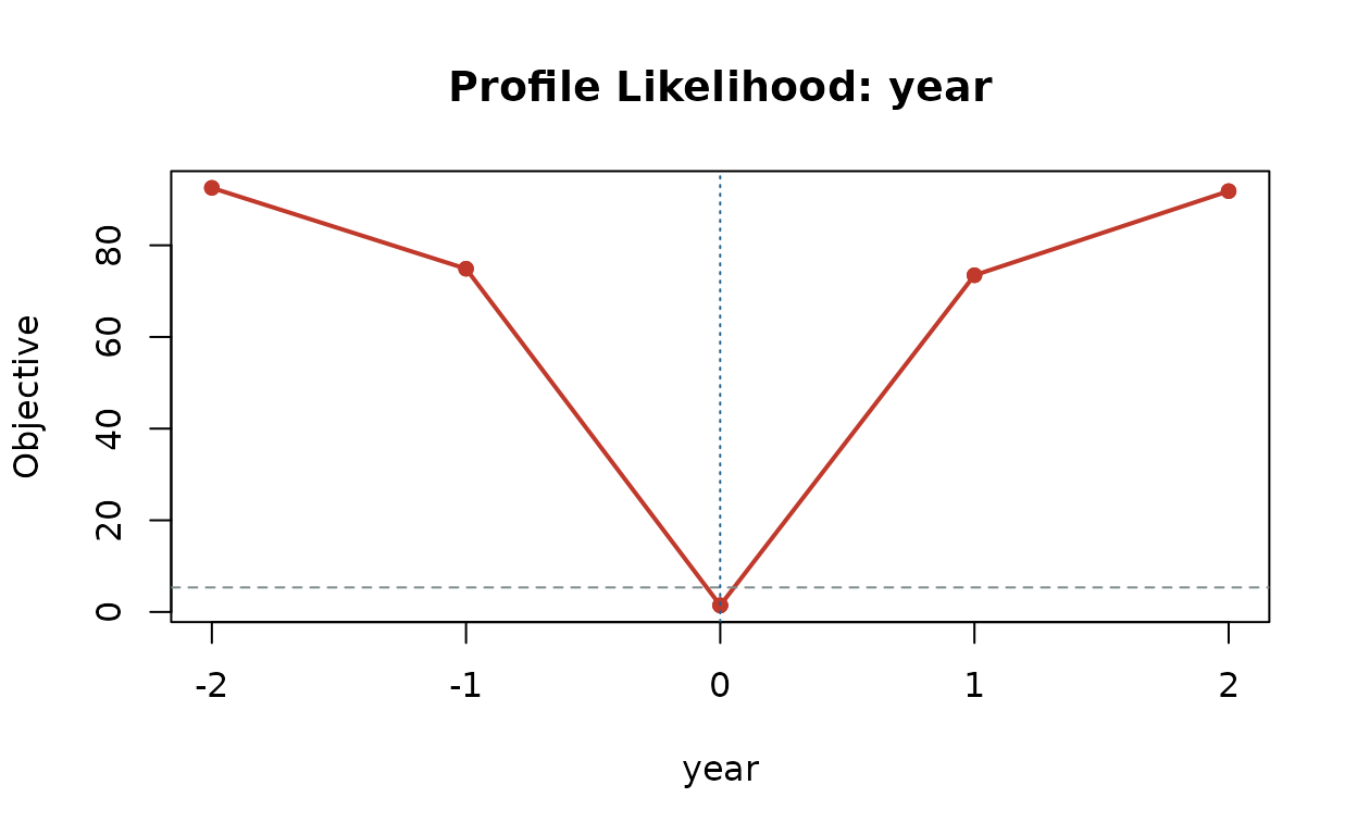

plot(pr, parameter = "tau1")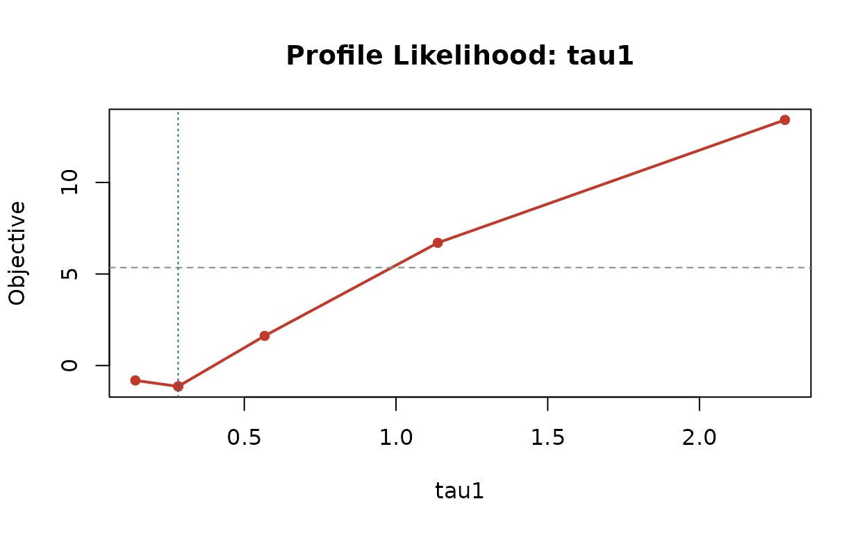

Custom Grids

For short vignettes, examples, or sensitivity checks, pass an explicit grid. Named grids are matched to the requested parameter names.

pr_grid <- profile_likelihood(
  fit_bcg,
  parameters = c("year", "tau1"),
  grid = list(
    year = c(-0.01, 0, 0.01),
    tau1 = c(0.1, 0.2, 0.3)
  )
)

pr_grid$summary
#>   parameter parameter_index           mle   cutoff ci_lower ci_upper
#> 1      year               2 -0.0003590629 5.349309       NA       NA
#> 2      tau1               3  0.2819106893 5.349309       NA       NA
pr_grid$profiles$tau1
#>   parameter parameter_index parameter_value  objective converged
#> 1      tau1               3             0.1  0.7020273      TRUE
#> 2      tau1               3             0.2 -1.4087885      TRUE
#> 3      tau1               3             0.3 -1.0108233      TRUE

Two-Dimensional Surfaces

Set parameter_pairs to request a two-dimensional profile surface. The surface is a contour plot of the same deviance-scale objective after fixing both parameters and re-optimizing the remaining parameters. The example uses a very small grid for speed.

In the contour plot below, points near lower contour values are better supported by the data. Moving outward from the minimum shows combinations of year and tau1 that require a worse model fit, even after the intercept is re-optimized.

pr_surface <- profile_likelihood(
  fit_bcg,
  parameters = c("year", "tau1"),
  parameter_pairs = list(c("year", "tau1")),
  n_points = 4,
  span = 2
)

names(pr_surface$surfaces)
#> [1] "year__tau1"
pr_surface$surfaces$year__tau1$parameters
#> [1] "year" "tau1"
dim(pr_surface$surfaces$year__tau1$objective)
#> [1] 5 5

plot(pr_surface, parameter = c("year", "tau1"), type = "contour")

Random-Effects Convenience Wrapper

profile_random_effects() is a focused wrapper for variance-component profiles. It returns the same confidence-interval summary idea, with profile data columns named around tau.

pr_tau <- profile_random_effects(
  fit_bcg,
  tau_indices = 1,
  n_points = 5,
  span = 2
)

pr_tau$summary
#>   tau_index       mle   cutoff ci_lower  ci_upper
#> 1         1 0.2819107 5.349309       NA 0.9858376
pr_tau$profiles$tau1
#>   tau_index tau_value objective converged
#> 1         1 0.1409553 -0.814914      TRUE
#> 2         1 0.2819107 -1.142022      TRUE
#> 3         1 0.2827391 -1.136381      TRUE
#> 4         1 0.5671398  1.619323      TRUE
#> 5         1 1.1376125  6.701402      TRUE
#> 6         1 2.2819107 13.415105      TRUE

Use profile_likelihood() when you want fixed effects, random effects, or 2D surfaces. Use profile_random_effects() when you only need quick random-effects profiles.