Profile Likelihood for mars Models
profile_likelihood.RdCompute one-dimensional profile-likelihood curves and confidence intervals for selected parameters by fixing one parameter at a time and re-optimizing the remaining parameters.
Usage
profile_likelihood(
  object,
  parameters = NULL,
  level = 0.95,
  n_points = 21,
  span = 3,
  grid = NULL,
  optim_method = "L-BFGS-B",
  control = list(factr = 1e+07, maxit = 400),
  parameter_pairs = NULL
)
Arguments
- object
A fitted
marsorpub_biasobject.marsprofiling currently excludes LASSO fits.- parameters
Optional parameter specification. May be
NULL(default: all random-effects parameters), numeric indices into the optimizer parameter vector, or parameter names. Fixed-effect parameters use the column names ofobject$design_matrix; random-effects parameters use namestau1,tau2, ....- level
Confidence level for profile-likelihood intervals. Default
0.95.- n_points
Number of grid points used per profiled parameter. Default
21.- span
Multiplicative span around the MLE for automatic grids. Default
3.- grid
Optional custom grid specification:
numeric vector: reused for each parameter
named list of numeric vectors keyed by parameter name
unnamed list of numeric vectors with one entry per profiled parameter.
- optim_method
Optimization method passed to
optim(). Default"L-BFGS-B".- control
Control list passed to
optim()for each conditional fit.- parameter_pairs
Optional 2D parameter-pair specification. May be a character vector of length 2, a numeric vector of length 2, or a list of such pairs.
Value
A list containing per-parameter profile grids and profile-likelihood
confidence intervals. The profiles component contains one data frame per
one-dimensional profile. The surfaces component contains optional
two-dimensional grids with x, y, objective, converged, and cutoff
entries.
Details
The profiled objective is reported on a deviance-like scale. For standard
mars models this is the fitted objective, equivalent to -2 log L up to
constants that do not depend on the profiled parameters. For publication-bias
models the same -2 log L scaling is used. Lower values therefore indicate
better-supported parameter values.
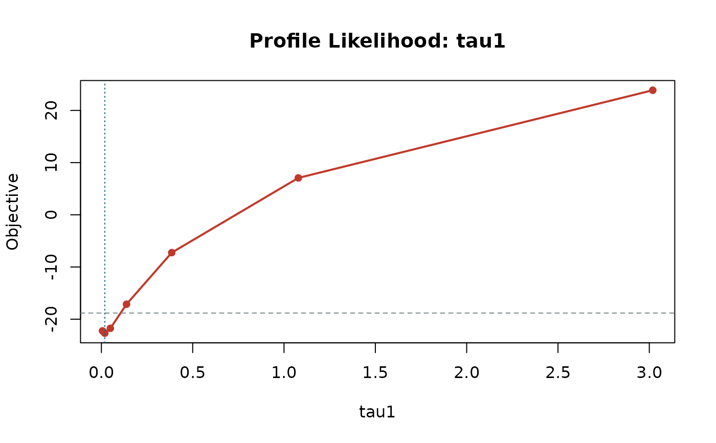
For a one-dimensional profile, the x-axis is the fixed value of the selected
parameter and the y-axis is the deviance-scale objective after all remaining
parameters have been re-optimized. The profile-likelihood interval contains
values whose objective is no more than qchisq(level, df = 1) above the
fitted minimum.
For a two-dimensional profile surface, the x- and y-axes are the two fixed
parameter values and the contours show the deviance-scale objective after all
other parameters have been re-optimized. The cutoff contour uses
qchisq(level, df = 2) above the fitted minimum and can be interpreted as an
approximate joint confidence region for the parameter pair.